A different indicator
Using an unusual indicator to inform a strategy that delivers 21% annual returns since 2004
The idea
"Mathematical reasoning may be regarded rather schematically as the exercise of a combination of two facilities, which we may call intuition and ingenuity.” Alan Turing.
It's hard to find anyone in Computer Science who doesn't hold Alan Turing in deep admiration. Widely regarded as the father of modern computing, Turing's groundbreaking work during World War II on breaking the Enigma code changed the course of history and laid the foundation for the development of the digital computer. His contributions to artificial intelligence, including the concept of the Turing Test, continue to influence the field today. Beyond his intellectual achievements, Turing was also an accomplished marathon runner, a lesser-known fact about this great genius.
Turing’s best marathon time was 2 hours, 46 minutes, 3 seconds, which was only 11 minutes slower than the winner in the 1948 Olympic Games. In fact, in a 1948 cross-country race, he beat future Olympic silver-medalist marathoner Tom Richards.
Although his best time might not be impressive by today's standards, it was an extraordinary achievement during the 1940s and 50s, highlighting his remarkable physical and intellectual prowess.
Since Turing's era, marathon completion times have decreased by 20%, or close to half an hour. This is an eternity. Several factors have contributed to the dramatic decrease in marathon times over the decades, such as improvements in nutrition, footwear technology, and overall sports science. However, I would like to highlight one particular change: the advancement in training protocols, particularly those focusing on VO2 max.
VO2 max is an indicator of the maximum rate of oxygen consumption during intense exercise. The concept of VO2 max became more widely understood and integrated into athletic training after the 1950s, leading to more scientifically driven training methods. Before that, training protocols were built using other indicators, which was suboptimal. Adopting a new indicator unlocked a significant performance improvement, leading to the current incredible marathon times.
This week, we will create a mean reversion strategy that outperforms the S&P 500 by trading its constituents based on a new signal. This new signal is not derived from RSI, one of the most used mean reversion indicators, nor the QPI, an indicator we created a while ago. We will base our strategy on a new indicator: the David Varadi Oscillator (DVO).
Here is the plan we will follow:
First, we will explain what is the David Varadi Oscillator and show how it is computed;
Then, we will prove its edge statistically and compare it with RSI's edge;
Finally, we will derive a strategy based on it and backtest it.
The David Varadi Oscillator
The Varadi Oscillator (DVO) is a leading indicator first proposed by David Varadi and originally aimed to reduce the influence of the trend component in oscillators. The DVO can be described as a rolling percent rank of detrended prices over a particular lookback period.
It has been proven useful to generate mean reversion signals, replacing the RSI and not being correlated to it.
The detrending process used for the DVO computation is simply the SMA of the ratio between the closing price and the average between the high and the low prices.
As you know, I usually don't share code. However, in this case, I believe it's easier to explain what this indicator does by looking at its Python implementation. It takes three lines:
This is the 2-period version, or DV2, equivalent to the 2-period RSI (or RSI2). While researching this article, I found a few slightly different definitions. This is the one we will use.
Now, let's see how much edge we can derive from it.
The edge
To assess the edge, we will look into all events when stocks' DV2 plunged below 10 while the stock's closing price was above its 200-day SMA. What would have happened if we had bought all these events and held them for 5 days? As a universe, we will look into all current and past Russell 3000 constituents (a bit over 10K symbols).
Here are the highlights:
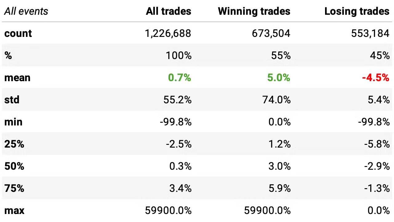
The mean return of buying any given stock whenever its DV2 is below 10 and holding for 5 days in a bull market is +2.0%;
54% of these events return positively, with a +7.6% expected return per trade;
46% of the trades were negative, with a -4.7% expected return per trade;
Looking at the high standard deviation and the distribution extremes, we see that it has fat tails. As such, it's good to look at the median values (so we can reduce the effect of outliers). Even at median values, the expected return is positive (+0.3%).
Now, let's look at non-events: the stats of what would have happened if we had bought all occurrences when the stock's DV2 was above 10 while its closing price was above its 200-day SMA:
We see worse expected returns (either in the mean or median values) and a worse win rate (52% vs. 54%).
The P-value is 0.017, below 0.05: the means of the two distributions are significantly different. So, we have an edge.
Comparing to DV2 to RSI2
Now, let's compare the edge of the DV2 indicator to the RSI2 indicator. First, let's look at what would have happened if we had bought all occurrences when the stock's RSI2 was below 10 while its closing price was above its 200-day SMA:
The median expected returns and win ratio are pretty close. The edge has about the same magnitude. Does it mean we are capturing the same opportunities?
To answer this question, let's look at how the events overlap:
As we see above, only 1 in 5 opportunities coincide (i.e., events where we have both DV2 < 10 and RSI2 < 10). Thus, although we have edges of similar magnitude, most of the events differ. In other words, buying stocks when their DV2 falls below 10 and expecting them to revert back to the mean is different than buying them when their RSI2 falls below 10 most of the time.
The impact of volatility
Now, let's compute how this edge varies with respect to volatility, measured as (normalized) Average True Range.
As expected, the higher the volatility, the higher the expected return in these short-term mean-reversion trades. (Outliers in both tails contaminate the 10th decile, but the conclusion holds still.)
Now, let's formulate a strategy to exploit this edge.
The strategy
At the opening of every trading session:
We will split our capital into 10 slots and buy stocks whose DV2 from the previous day closed below 10;
If there are more than 10 stocks in the universe with the entry signal triggered, we will sort them by Normalized Average True Range and prioritize the high-volatility stocks;
We will hold 10 positions maximum at any given moment;
When the stock closes above yesterday's high, we will exit on the next open;
We will only trade S&P 500 constituents (at the specific past date).
Just to reinforce: we use Norgate data, a survivorship bias-free dataset. It also has the evolution of S&P 500 constituents over time, enabling us to prevent selection bias.
Experiments
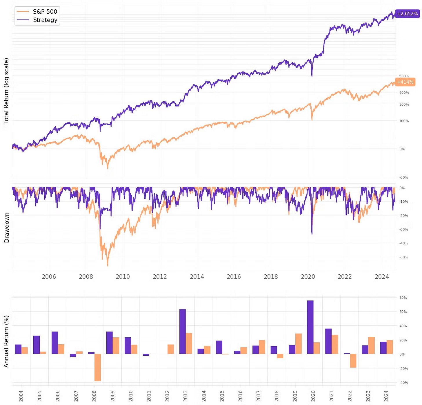
First, let's check how the strategy would perform as described.
Not bad for a first experiment. Here are the highlights:
The strategy delivers a 17.4% annual return, over twice the benchmark during the same period;
Sharpe ratio is 0.87 vs. 0.51 from S&P 500;
The maximum drawdown is at 34%, much better than the 57% from the benchmark, but still too high for most investors;
The strategy trades 475/year on average, or approximately 2x/day, with a win ratio of 64.8%;
The expected return per trade is +0.36%, with a low payoff ratio of 0.69.
Let's look at the backtest of the strategy with an entry signal based on RSI2 instead of DV2 as the only difference to compare:
All metrics are pretty similar. Analyzing the daily returns and the individual trades from both strategies, we observe some interesting facts:
The correlation between the daily return streams is 80%. This high value explains why the overall metrics are so similar;
The intersection between the 9,844 trades from the DV2 strategy and the 10,013 trades from the RSI2 strategy is only 1,252, or 6.7%, as seen in the chart below. This means that, although there is a high correlation between the returns, the strategies are executing different trades.
Now, let's see how we can improve the DV2 strategy.
Improving the signal
So far, the strategy's entry signal is based on two simple conditions:
A stock (from S&P 500 universe) must have its DV2 indicator below 10;
It also must have its closing price above its 200-day SMA to ensure we are trading bullish stocks.
Now, let's add a third condition: we will only trade stocks with a positive return in the past six months.
Let's analyze the results:
Adding this third condition brought a nice improvement:
The annual return is now at 20.9%, over +3ppts above the previous result;
Sharpe ratio achieved 1.01, vs. the previous 0.87;
Maximum drawdown remained about the same;
Looking at the trade statistics, we see that all key metrics improved: expected return per trade, win ratio, and payoff ratio.
Now, let's look at the month-by-month returns:
If we had traded this strategy since 2004:
We would have had only one down year in 21;
We would have seen 64% of the months positive, with the best at +36.7% (Nov’20);
We would have seen 36% of the months negative, with the worst at -12.7% (Mar'20);
The longest positive streak would have been 11 months, from Dec'12 to Ocr'13;
The longest negative streak would have been 4 months, from Mar'17 to Jun'17.
The impact of slippage and trading costs
Finally, let's check the impact of trading costs on the results:
As expected, the higher the trading costs, the lower the returns.
Final thoughts
There are so many ways to measure different phenomena. Using DV2 instead of the usual RSI2 resulted in profitable tests. Although the correlation between their return streams was high (80%), the intersection between trades was low enough (6.7%) to keep us interested in studying strategies informed by DV2.
Would I trade this strategy as is? Not really. A 34% maximum drawdown is too high for most investors. Nevertheless, we should continue to explore ideas using unusual indicators such as DV2. Some potential improvement areas:
Adding a short leg and trading a long & short system;
Mixing a strategy based on DV2 with a strategy based on RSI2 in order to improve the risk-adjusted returns;
Mixing different parameters (both the threshold and the lookback), doing something similar to what we did in the Trading the Mean Reversion Curve article.
I'd love to hear your thoughts about this approach. If you have any questions or comments, just reach out via Twitter or email.
Cheers!


Hi, first off all want to say that I loved the article! I'm building the strategy you talk about here as my first project. Do you have any other suggestion for an exit strategy. I fell that some upside potential is being cut with the exit strategy you use here. Thanks!
Pretty cool seeing those Vann Diagrams. Kamala would be proud. Have you tested to see if the trades (mean returns) in the intersection of the Venn Diagram are different from the mean returns in non-intersecting circles? One would think intersection trades should have a higher win rate, since they have 2 successful signals supporting them.