

The idea
“The biggest risk is that you have a losing strategy when you think you have a winning one.” Jeff Yass
Last month, while listening to Annie Duke’s TED Talk about risk, I learned the quote above from Jeff Yass, founder of Susquehanna International Group.
Annie is a former professional poker player turned author and decision-strategy consultant. Her famous book, Thinking in Bets (2018), is a great read! In it, she argues that most decisions are made under uncertainty, so we should treat them like a poker player treats a hand: as bets with probabilities, not as right-or-wrong choices. She also has a Substack worth subscribing to.
Yass was himself a serious poker player who spent time at the Las Vegas tables before (and after) founding SIG. We could say Annie’s “think in bets” framework is essentially the house philosophy Yass built SIG on.
Back to the idea… I loved the quote about how Jeff summarized this truth: the greatest risk is fooling yourself, believing your strategy wins when it really loses.
Do we have a winning strategy or a losing strategy?
While researching, if you believe you discovered a winning strategy right off the bat, your cognitive biases might get you into trouble. Conversely, if you truly believe your models are wrong (they are), your belief might actually help you.
If we assume we are right, confirmation bias will kick in and do its job. Our goal will be to prove we are right. And we are so easily fooled…
If we assume we are wrong, though, we have a more useful mindset. Our goal, then, is to be less wrong. We aspire to be less wrong. We look at our work and ask, “How is this wrong? How can I make it less wrong?”
This week, we will implement the paper Twin Momentum: Fundamental Trends Matter, by Dashan Huang, Huacheng Zhang, and Guofu Zhou (2021).
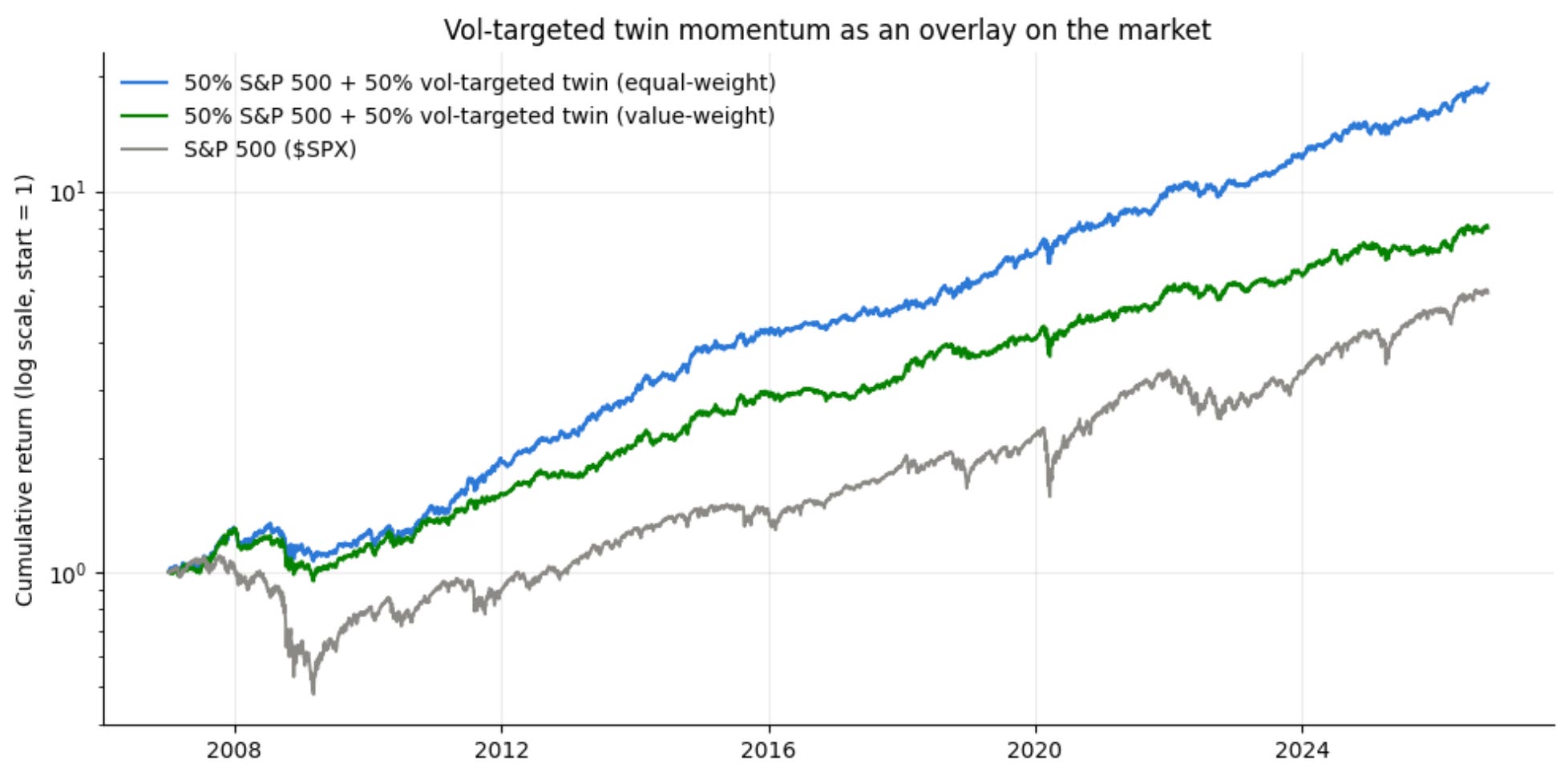
Here’s the plan we will follow:
First, we will quickly summarize the paper
Next, we will share our vanilla implementation
Then, we will implement some improvements
Finally, we will close as usual with final thoughts and next steps
I’ll share the code with paid subscribers at the end of the article. If you enjoy the work, consider becoming a paid supporter!
Paper summary
Twin Momentum: Fundamental Trends Matter, by Huang, Zhang & Zhou (2021), has a pretty simple idea: intersecting two nearly uncorrelated sources of return predictability:
Price momentum: the classic 12-to-1-month past return
Fundamental momentum: the fundamental implied return (FIR)
The fundamental implied return (FIR) is a monthly cross-sectional forecast built from seven quarterly fundamental signals and their 1/2/4/8-quarter trends.
The seven fundamental variables are:
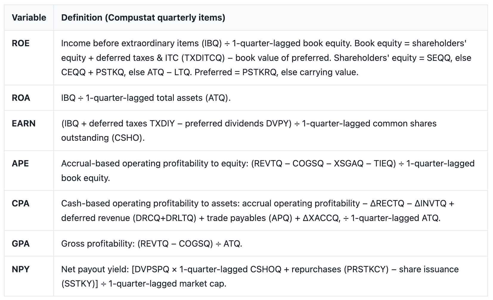
From these fundamentals, the authors create 28 predictors per stock: moving averages over L = 1, 2, 4, 8 quarters. Then, FIR is the monthly cross-sectional regression of returns on the 28 predictors. Applying the fitted slopes to current values gives a real-time forecast of next month’s return.
Finally, to implement the Twin Momentum strategy, at each rebalance date (the last day of the month), we run independent 5x5 double sorts on price momentum and FIR and go long on top ∩ top and short bottom ∩ bottom.
The authors achieved a +1.81%/mo (t = 4.5) return, which is more than the sum of the independent parts (they compared it with a pure price momentum strategy and a pure FIR strategy). This result was unexplained by the main academic factor models (CAPM/FF3/FFC/HXZ/FF5). Interestingly, the authors showed this result was driven by the long leg and survived size/cost/sentiment checks.
Vanilla implementation
The authors used quarterly Compustat accounting data (1973:01–2019:06) and monthly CRSP data (1976:05–2019:07). I got good results with Sharadar with small adjustments (code details at the end).
Whenever using fundamental data, it’s important to use point-in-time, as-reported numbers. Using restated figures or considering numbers earlier than when they were effectively reported by companies is an easy way to introduce lookahead bias.
The results below show four variants:
Equal-weights, vanilla
Equal-weights, vol-targeted
Value-weights, vanilla
Value-weights, vol-targeted
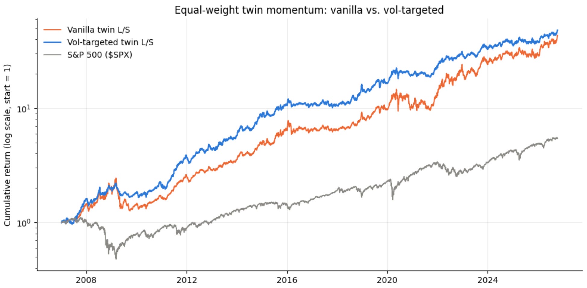
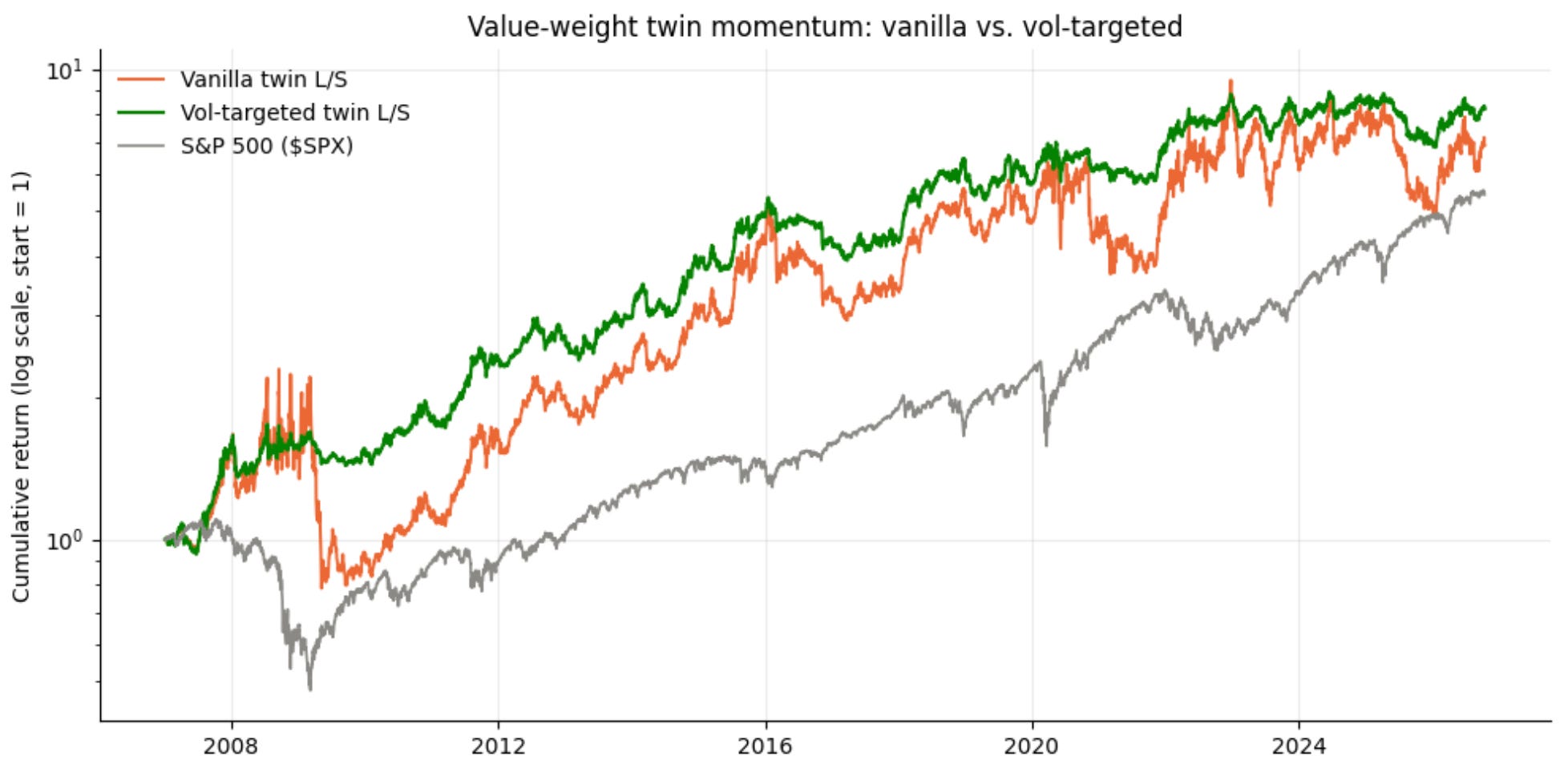
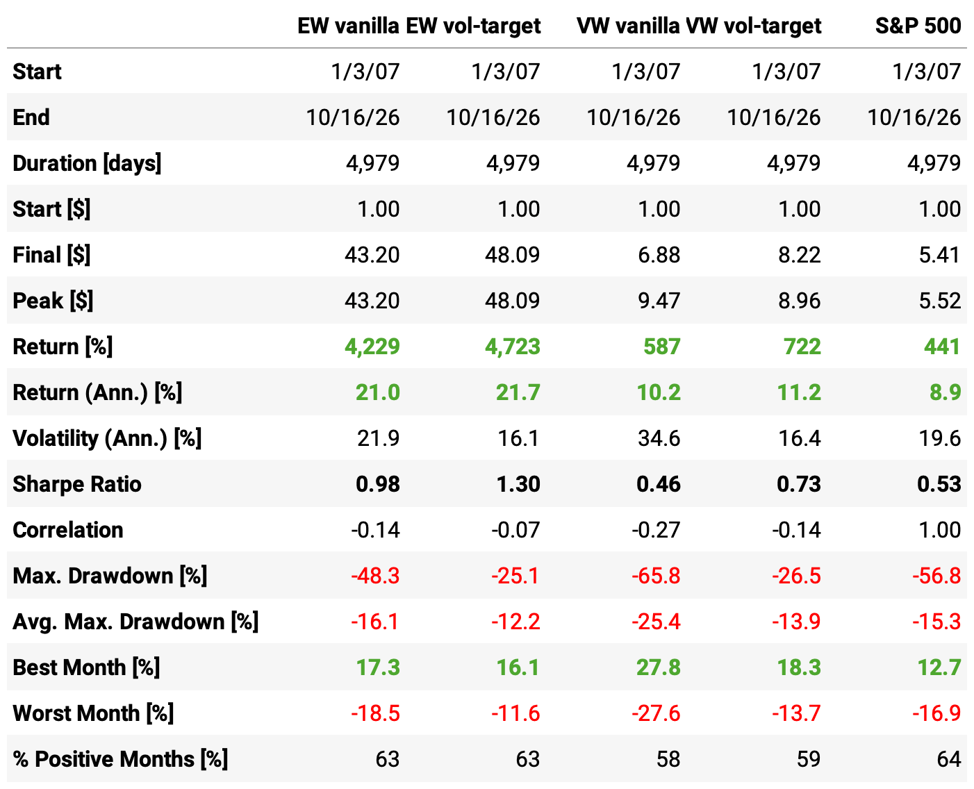
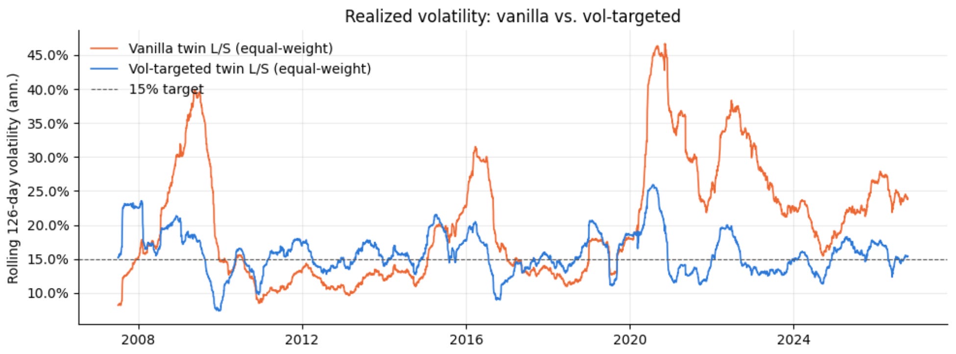
First, we notice the benefit of volatility targeting. We can see it even better by plotting the rolling volatility:
Next, let’s look at the performance numbers. The table shows that, although positive, the numbers are not impressive (especially since costs are not yet included). However, one number pops out of the table: the slightly negative correlation with the market.
A naive 50/50 allocation between the vol-targeted strategy and the S&P 500, rebalanced once a year, produces the following results:
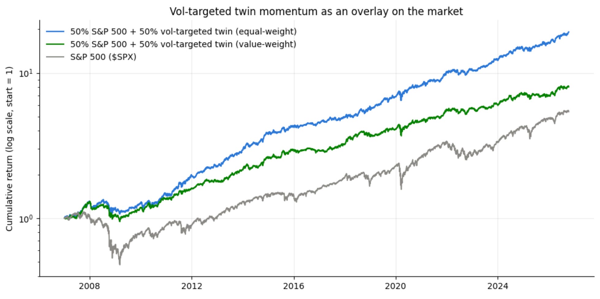
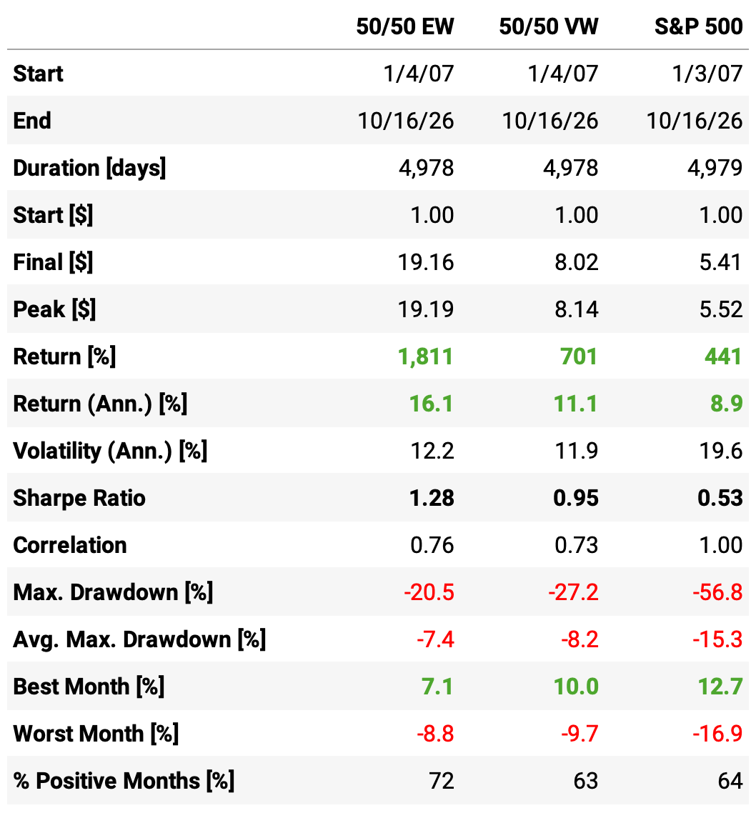
As expected, the equity curves and the numbers benefit from the diversification: blending uncorrelated return streams is always good.
Now, let’s pause and ask: is this a winning strategy, or a losing strategy in disguise? How are the numbers above wrong? And most importantly: how can we make them less wrong?
Liquidity and cost
Equal-weight results are dominated by small, illiquid, expensive-to-trade names where mispricing tends to be strongest, as small caps vastly outnumber large caps. Value weighting measures whether the effect holds where the money actually is: big, cheap-to-trade stocks that can absorb capital. Thus, a good first step in the less-wrong direction is to consider the value-weighted version as our base case.
Next, we can also restrict our tradable universe to names with a minimum ADV (e.g., $500k), a minimum price to avoid penny stocks (at least $1.00), and avoid hard-to-trade types (e.g., SPACs). Finally, we must consider trading costs. 5 bps/side is a good place to start.
Here are the results for the pure Twin Momentum strategy:
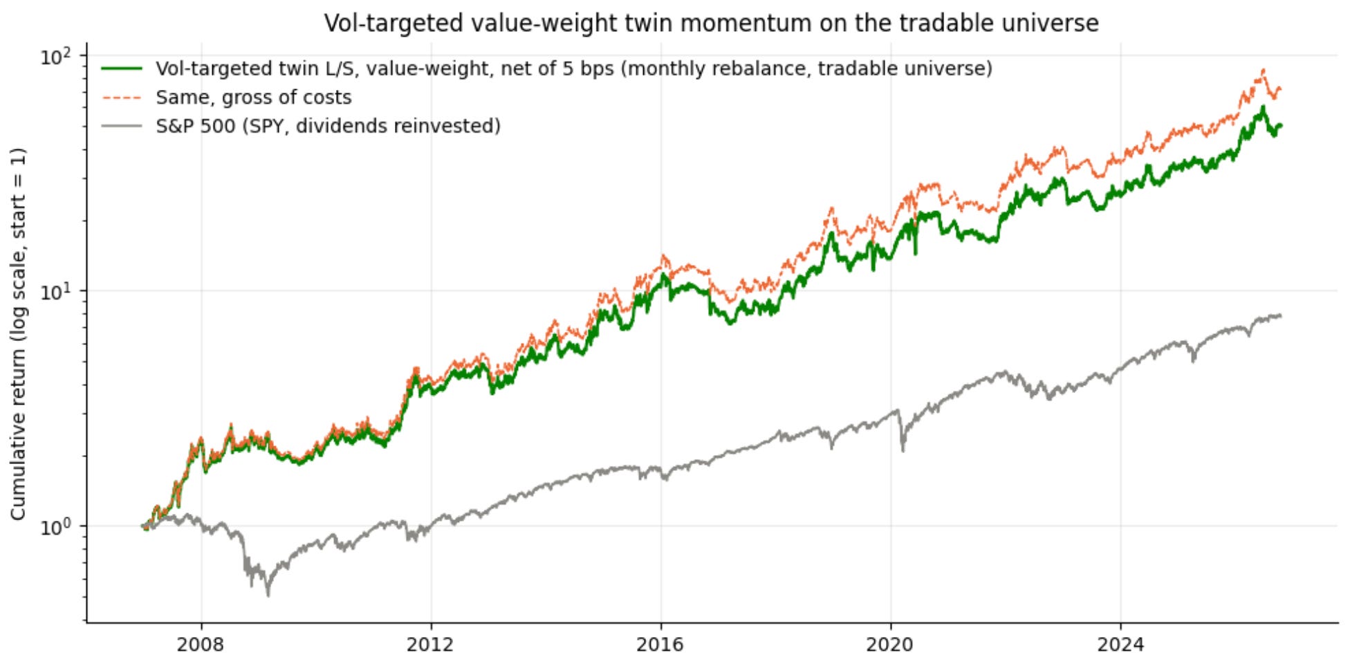
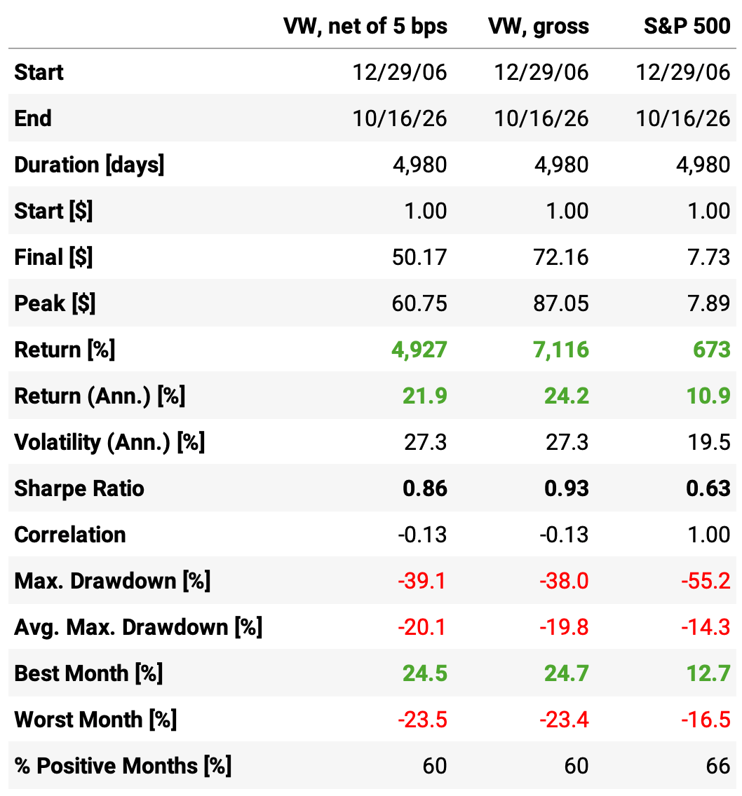
These numbers beat the benchmark, but they're still not amazing. However, they are less wrong than what we were seeing before. Now, as we noticed the negative correlation with the market, let's see what a 50/50 book with the strategy and the S&P 500 delivers:
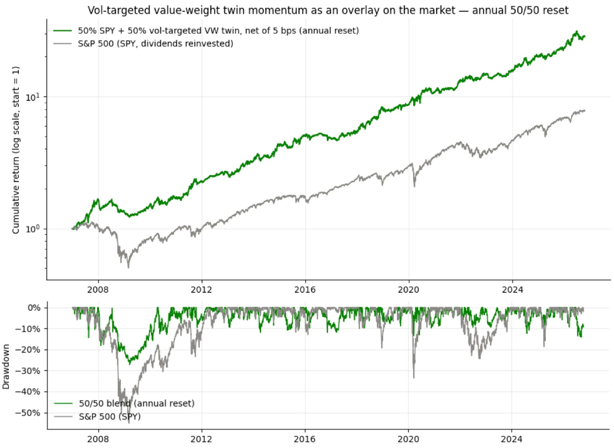
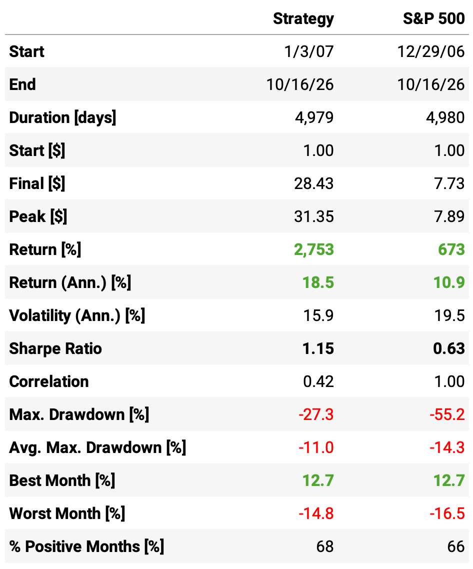
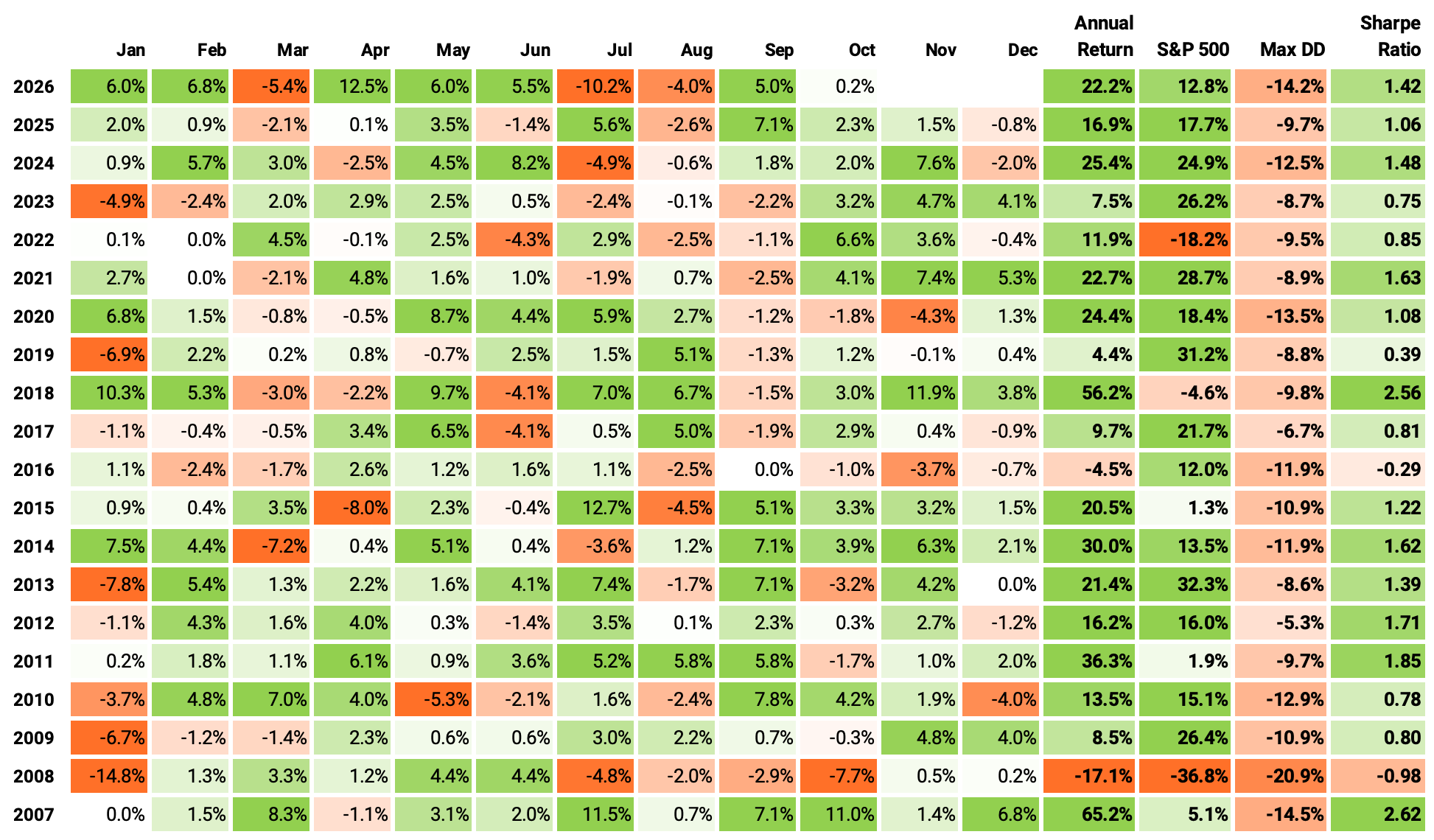
There we have it. Our strategy shows a Sharpe of 1.15, about 2x the benchmark, with approximately half the max drawdown. Not bad for such a simple idea.
Final thoughts
So, is Twin Momentum a winning strategy or a losing one in disguise? Honestly, we still don’t know for sure. What we do know is that our numbers are less wrong than when we started.
The vanilla implementation looked fine at first glance: positive returns and a slightly negative correlation with the market. But the equal-weighted version leaned on small, illiquid names that are expensive to trade, and we hadn’t paid a single basis point in costs. So we corrected course. We made value weights the base case, restricted the backtest to a tradable universe (minimum ADV, minimum price, no SPACs), and charged 5 bps/side in trading costs. The standalone numbers got humbler, but also more honest. Blended 50/50 with the S&P 500, the strategy delivered a 1.15 Sharpe ratio, roughly twice the benchmark’s, with about half the max drawdown.
Does this mean we found a winning strategy? Not yet. There’s still plenty that’s wrong with these numbers:
Shorting isn’t free: borrow fees and hard-to-borrow names aren’t in the backtest yet, and 5 bps/side may be optimistic for the short leg;
The long leg does the heavy lifting: the authors found the alpha concentrated there, so a long-only or beta-hedged version deserves a test;
Out-of-sample decay: the paper’s sample ends in mid-2019, so everything after that is out-of-sample and worth isolating;
A smarter FIR: the fundamental forecast is a plain linear regression on 28 predictors, which makes it a natural candidate for regularization or non-linear models;
Robustness: we should check sensitivity to the number of buckets, the rebalance date, and the blend weights (a naive 50/50 rebalanced once a year is a starting point, not an answer).
Jeff Yass’s warning is a good one to keep pinned above the desk. The danger was never that our models are wrong, because they always are. The danger is forgetting it. Every step in this article started with the same question: how is this wrong? That question won’t turn a strategy into a winner. But it’s the best defense we have against falling in love with a loser. Or, as Annie would put it, we don’t need certainty, just better bets.
So let’s keep aspiring to be less wrong.
As always, I’d love to hear your thoughts. Feel free to reach out via Twitter or email if you have questions, ideas, or feedback.
Cheers!