

The idea
“If I have seen further it is by standing on the shoulders of Giants.” Sir Isaac Newton.
Isaac Newton was arguably the greatest scientist who ever lived. He effectively discovered gravity. He showed us how to predict the motion of the planets. He had every right to brag about his genius. Yet he chose humility. Why?
His critics paraded their ideas with hubris. Newton offered his with deference to those who came before. And that humility was no pose. It came from something he understood early and deeply: knowledge builds upon itself. Each idea improves on the last, little by little, until the small gains add up to something revolutionary. That is the essence of his most famous “standing on the shoulders of Giants” metaphor.
From a young age, Newton kept a commonplace book, a gift from his father. In it, he copied passages from what he read and added his own notes, turning borrowed knowledge into original ideas. He called it his “Waste Book.” The name was a nod to the usefulness of useless knowledge and the combinatorial nature of creativity, what Einstein would later call “combinatory play.” Creating by connecting was the foundation of Newton’s mind. It was his real superpower.
This week, we will cover two articles. We will build on The Modern Spirit of Statistical Arbitrage, a great piece by SysLS. And we will implement a recent breakthrough paper that rigorously tested more than 190 signals in the US equity market.
Here’s our plan:
First, we will summarize the modern spirit of stat arb.
Next, we will construct a signal and show, in a few lines of code, how it performs across several large baskets.
We will then present the combined performance of the top ~20 signals and walk through them, summarizing the source paper along the way.
Finally, we will lay out a simple way to merge these signals into a portfolio that survives friction and costs.
Let’s get started.
What is statistical arbitrage?
At its core, statistical arbitrage is a class of strategy built from a portfolio of signals. Each signal assigns weights to instruments based on how much they outperform or underperform the rest of their basket, measured against some central point of all the other instruments. This can happen in any space: returns, price, volume, flow, dividends, and so on. The basket is then built so that its net factor exposures tend toward zero, which means most of its returns come from idiosyncratic moves rather than broad market or factor exposure. It’s a broad definition, and that’s the point. It covers every flavor of stat arb.
For more details, check the great post by SysLS.
Let’s see a concrete example. We will start with Factor 46 from the paper we are sourcing the signals.
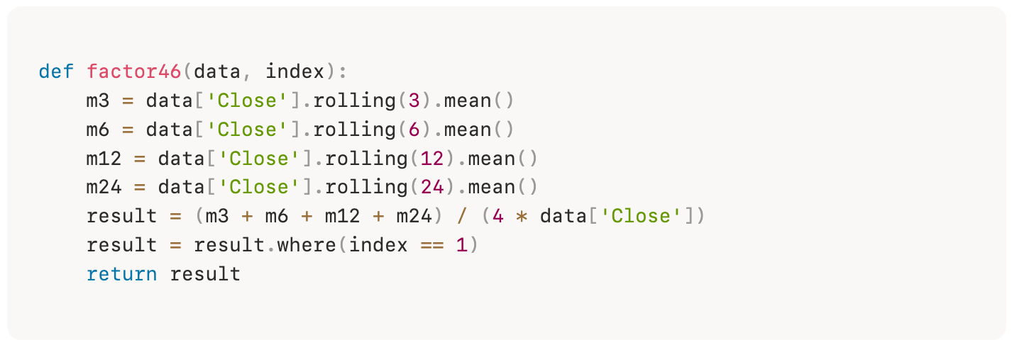
Definition. Factor46 is the paper’s Multi-Period Mean Reversion Ratio, computed as:
(MEAN(CLOSE,3) + MEAN(CLOSE,6) + MEAN(CLOSE,12) + MEAN(CLOSE,24)) / (4 * CLOSE)The Python code is straightforward:
The inputs are clear: both are date-indexed, point-in-time panels covering every symbol that has ever belonged to a given universe (the Norgate “… Current & Past” watchlist, so it’s survivorship-bias free):
data: a wide DataFrame whose columns are a two-level (’Feature’, ‘Symbol’) MultiIndex, so
data['Close']slices out a single date-×-symbol price matrix. Features available areOpen,High,Low,Close,Amount,Volume, andVWAP. factor46 only touchesdata['Close'].index: a same-shaped date-×-symbol integer DataFrame that is 1 on days a symbol was an actual index constituent and 0 otherwise. factor46’s final
result.where(index == 1)uses it as a membership mask, blanking out the factor value for any stock/day that wasn’t in the universe at that time so it can’t be traded.
As we can see, Factor 46 takes four trailing moving averages of the closing price (3, 6, 12, and 24 days, each window roughly doubling, spanning a few days out to about a trading month), equal-weights them into a single blended reference price, and divides by today’s close. The result is a pure ratio centered near 1:
a value > 1 means the current price sits below its own multi-horizon average (the stock has recently sold off relative to its recent history), and
a value < 1 means it sits above it (recently run up).
It is, in essence, a smoothed, scale-free “distance from fair value” measure where “fair value” is the stock’s own recent average price rather than any fundamental anchor.
What it captures and why economically. The effect is short-horizon cross-sectional mean reversion / contrarian price correction. The paper grounds this in behavioral universality: overreaction, herding, and liquidity-seeking are cognitive traits common to all market participants, so when traders push a price away from its recent path (chasing news or dumping inventory), the dislocation tends to correct. Crucially, arbitrageurs are slow to close these gaps because of noise-trader risk and limits to arbitrage, which lets the reversal premium persist long enough to be harvested.
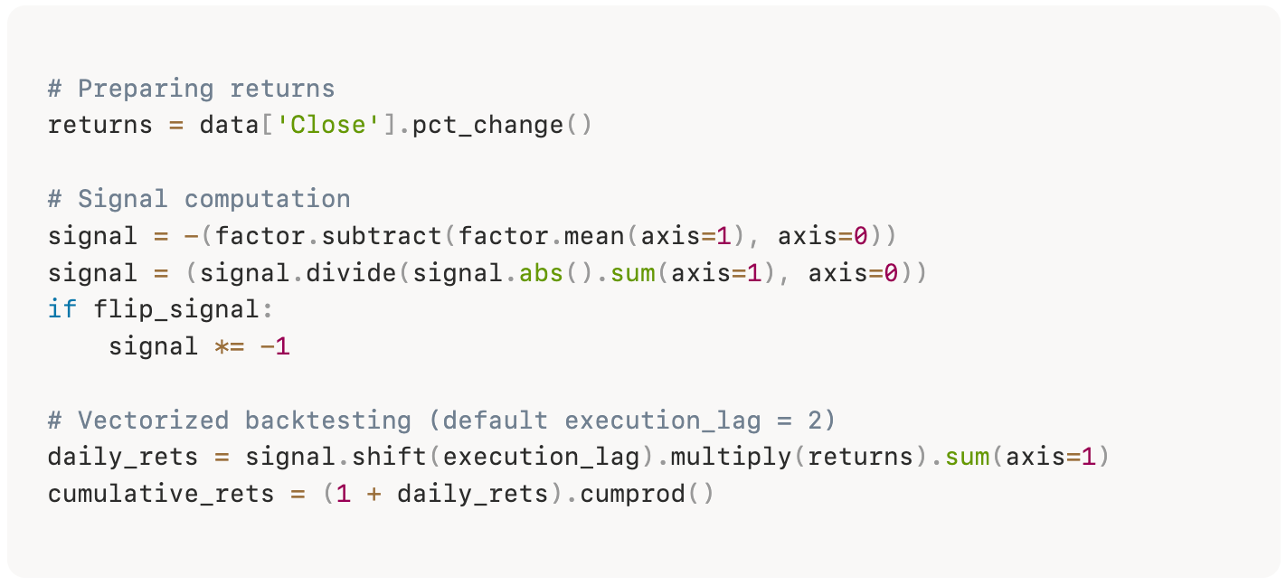
Now, let’s see the code that tests this signal. The most important lines are:
What is happening here?
The line signal = -(factor.subtract(factor.mean(axis=1), axis=0)) measures how far each stock sits from the center of its basket. For every day, it takes the cross-sectional mean of the factor across all stocks and subtracts it from each stock’s value. What’s left is each stock’s displacement from the group. The leading minus sign then flips the bet: stocks far below the average get positive weight, and stocks far above it get negative weight. That is the contrarian core of stat arb, betting that extremes revert toward the center.
The line signal.divide(signal.abs().sum(axis=1), axis=0) just normalizes. It divides every weight by the total gross exposure that day, so the book always sums to the same size and the longs roughly fund the shorts. This keeps the portfolio close to dollar-neutral and comparable across time.
The flip is optional. When flip_signal is true, it multiplies the whole book by -1, reversing the direction of every bet. This is useful because we don’t always know in advance which sign of a factor is the profitable one. The same formula can be tested both ways, longs and shorts swapped, without rewriting anything.
The last line runs the backtest: signal.shift(execution_lag).multiply(returns).sum(axis=1). It takes each day’s weights, shifts them forward by execution_lag days (two by default), and multiplies them by that day’s returns. The shift is the important part. It makes sure we only earn returns on positions we could have actually held, using yesterday’s signal to trade today rather than peeking at information we wouldn’t have had in time. Summing across all stocks then collapses the basket into a single daily P&L for the whole portfolio.
Let’s see the results:
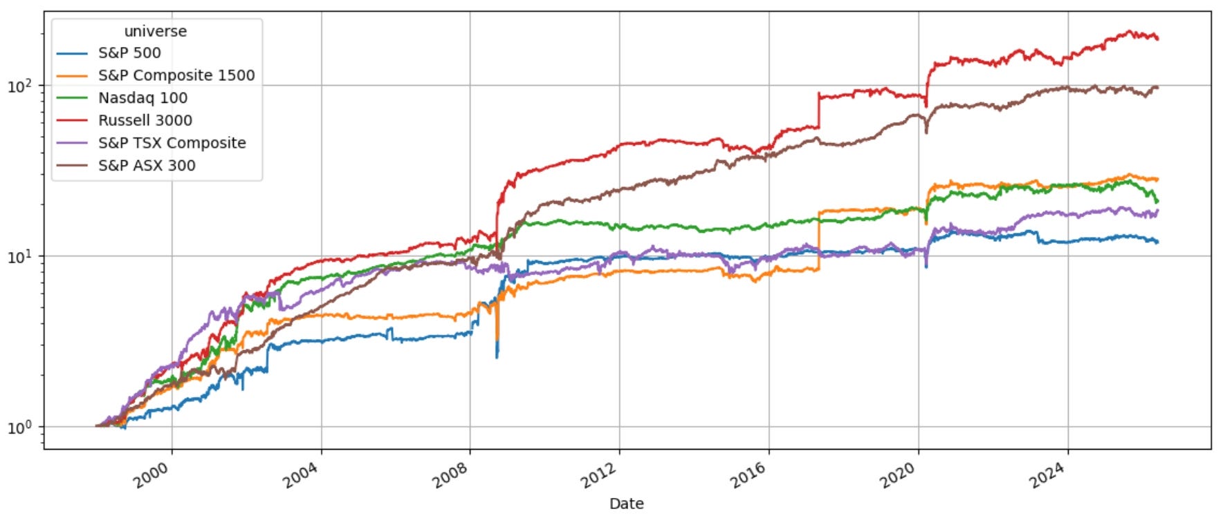
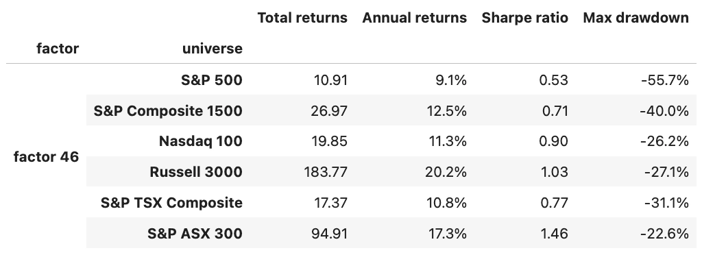
Factor 46 is encouraging, but on its own it’s not a finished strategy. The same formula behaves very differently depending on where we point it: a 0.53 Sharpe on the S&P 500, a 1.46 on the S&P ASX 300. The S&P 500 version is the clear laggard, with the weakest return and a brutal 55.7% drawdown that no one would want to sit through. And these numbers are gross of costs, so the real picture is worse. That’s the honest takeaway: a single signal, however clever, is rarely tradeable alone. The edge is real but thin, and one factor gives us no diversification when it goes through a bad stretch. The fix is to stop relying on any one signal. Combine many, each with its own small edge, and the weak spots start to cancel out. That is exactly where we go next.
From a single signal to a portfolio of signals
Let’s see what happens when we combine the strongest 17 signals according to the source paper:
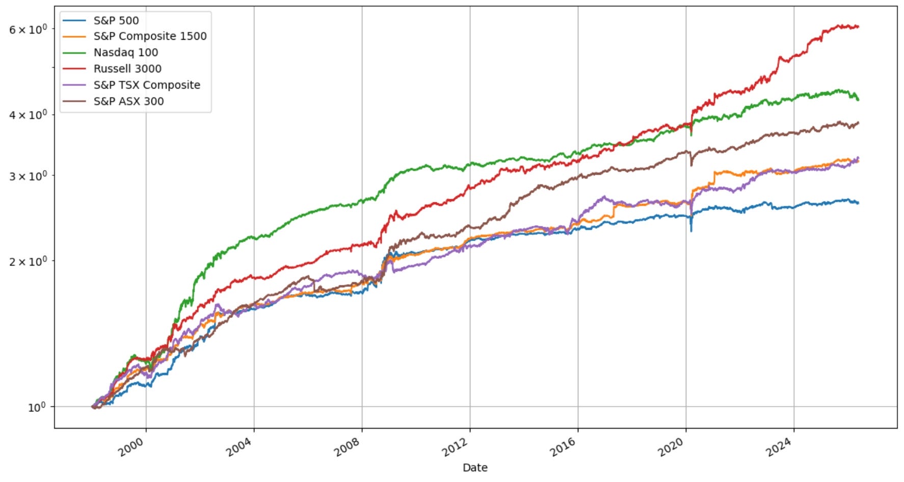
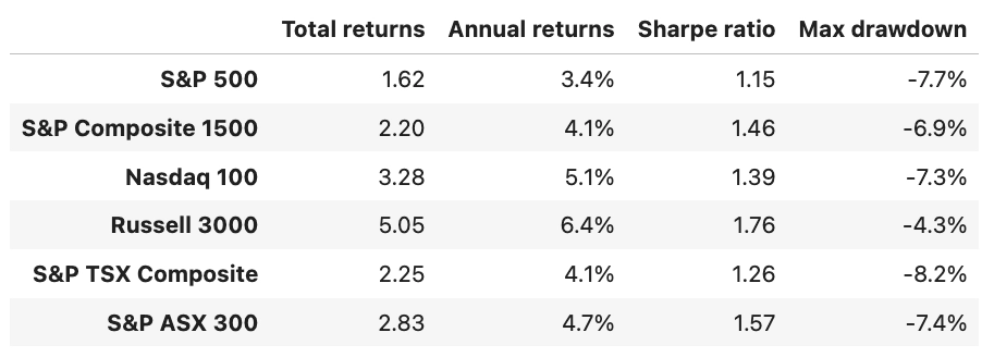
The effect of diversification is immediate. The single Factor 46 signal swung as deep as 55.7% on the S&P 500; the combined portfolio’s worst drawdown across all six universes is just 8.2%, and only 4.3% on the Russell 3000. Every Sharpe ratio now sits above 1.0, from 1.15 to 1.76, where the lone signal struggled to clear 0.5. The annual returns look smaller, but that’s the point: the single signal earned big numbers by running enormous risk, while the portfolio earns steadier returns with a fraction of the pain. That’s diversification doing its job. Seventeen small, imperfect edges combine into something far smoother than any one of them.
So what are these seventeen signals? Let’s look at them next.
Inside the portfolio
The list below shows the strongest signals, the most pervasive cross-sectional drivers according to the paper: