

The idea
“Networks are everywhere. All you need is an eye for them.” Albert-László Barabási.
Albert-László Barabási is a Romanian-born Hungarian-American physicist, renowned for his pioneering discoveries in network science. In his seminal 1999 paper with Réka Albert, “Emergence of Scaling in Random Networks,” he reshaped how we understand connected systems. His 2002 book Linked carried the argument to a general audience, making the case that networks are everywhere once you develop an eye for them.
This week, we will implement the paper Network Momentum across Asset Classes by Pu, Roberts, Dong & Zohren (2023), from the Oxford-Man Institute.
Using graph learning, the authors build a dynamic network across 64 futures contracts in 4 asset classes, then trade the network momentum that propagates through it:
1.51 Sharpe and 22% annual return, 2000-2022 (out-of-sample),
Only 65% correlated with classic momentum: a genuinely new signal, not a repackage,
Cross-class links are the edge: connecting bonds → currencies → commodities beats trading each class in isolation,
Networks stay remarkably stable, yet visibly reshuffle during the 2008 crisis and the 2020 crash.
No economic ties. No company data. Just prices, a graph, and a regression.
Here’s our plan:
First, we will quickly summarize the paper;
Next, we will implement the paper, step by step, showing our results throughout the journey;
Then, we will run some diagnostic analysis (turnover, costs, placebo, regime robustness), showing the signal survives;
We will then propose a signal-smoothing improvement to reduce turnover & costs;
Finally, we will wrap up with final thoughts and next steps.
Let’s get to it.
Paper summary
The big idea
Momentum spillover is the phenomenon where a “winning” asset’s momentum propagates to connected assets, suggesting you should go long assets linked to past winners and short those linked to past losers.
It was originally documented only in pairwise, fundamentally-linked pairs: a company’s stock and its bonds, or firms along a supply chain.
This paper coins network momentum: a signal for a target asset built by averaging the momentum features of its network neighbors, weighted by connection strength. The key leap is extending it across four asset classes at once: commodities, equities, fixed income, and currencies.
How it works
Universe: 64 liquid continuous futures contracts, spanning the four classes, 1990-2022.
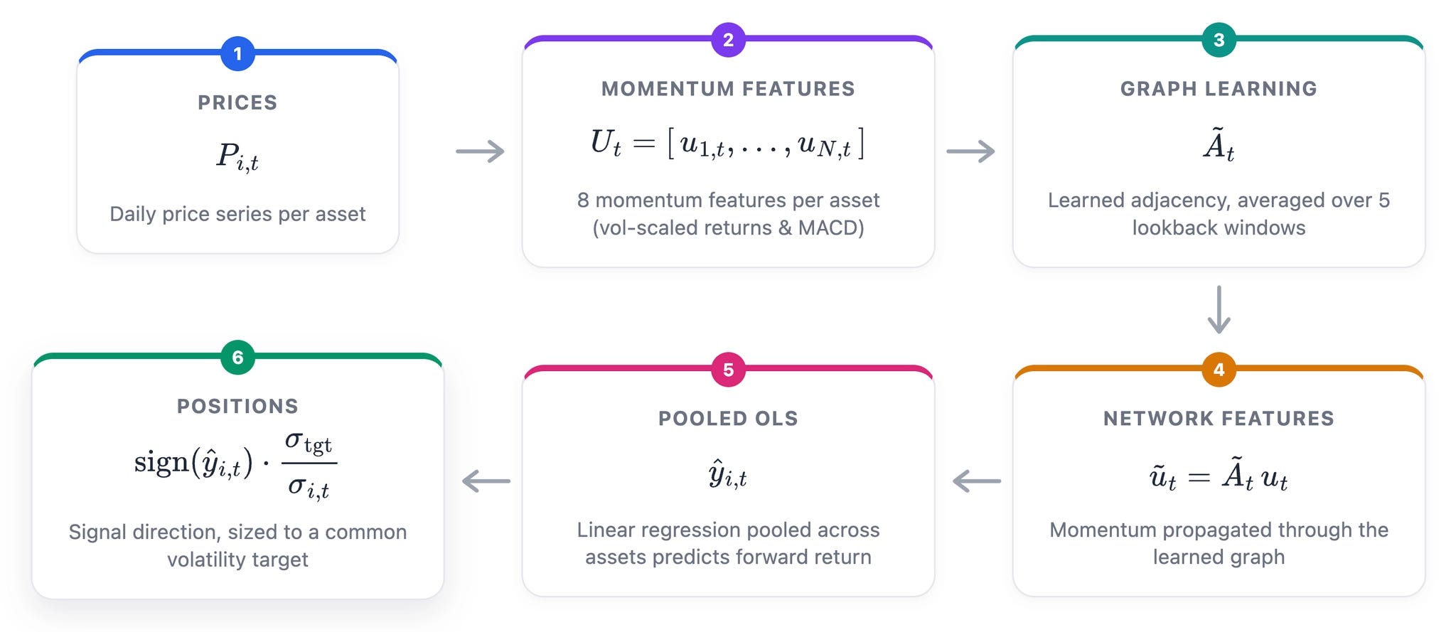
Features: 8 individual momentum features per asset: volatility-scaled returns over 1-day, 1-month, 3-month, 6-month, and 1-year horizons, plus 3 normalized MACD indicators at different time scales.
Graph learning: A linear, interpretable convex-optimization model estimates a daily adjacency matrix where each asset is a node and edge weights reflect similarity in momentum features (non-negative, sparse, no self-links). They ensemble five graphs from different lookback windows (252 to 1260 days) for stability.
Signal + portfolio: Network momentum features (neighbor-weighted averages) feed an OLS regression predicting each asset’s next-day volatility-scaled return. The long/short portfolio is called GMOM, with positions volatility-scaled to a 15% target.
Key results
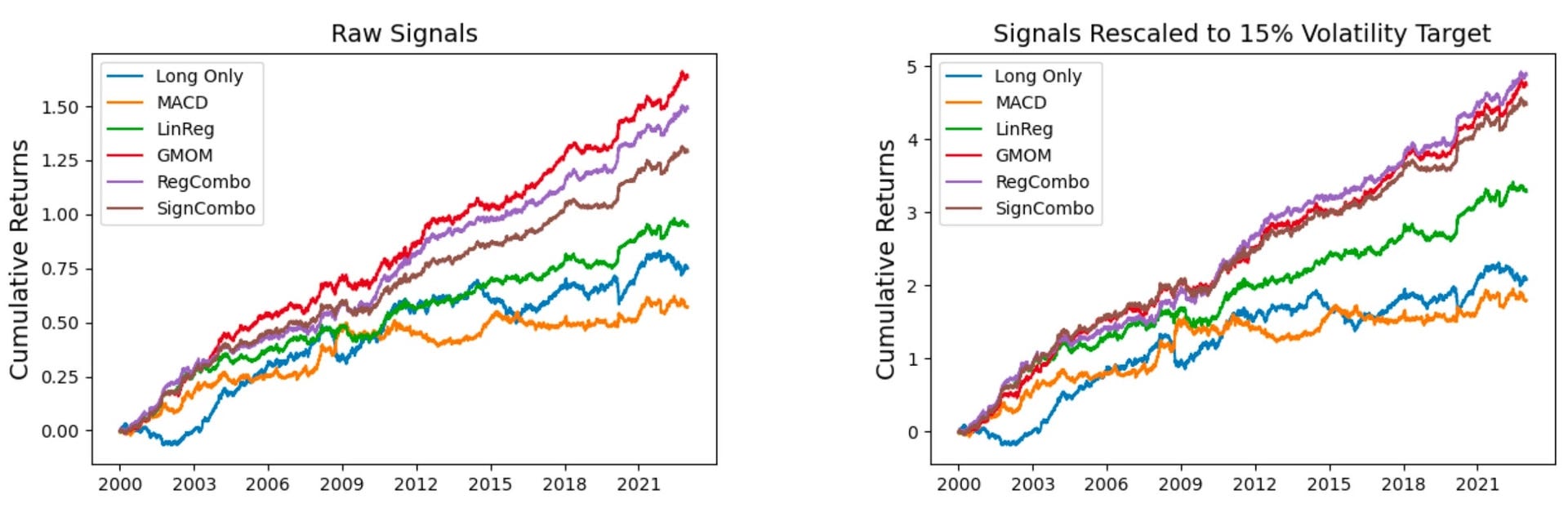
Sharpe ratio of 1.51 and ~22% annual return out-of-sample (2000–2022), after volatility scaling.
Beats every benchmark tested: Long-Only (0.73), MACD (0.70), and, critically, individual momentum / LinReg (1.13), despite using the exact same input information.
Also posts the smallest maximum drawdown (~20%) and shortest drawdown duration of the group.
Only ~65% correlated with individual momentum (72% sign agreement), meaning the network layer generates a genuinely new signal rather than repackaging classic momentum.
What makes it work (robustness)
Cross-class connections are the secret sauce. Restricting to a single class, or to intra-class edges only, degrades performance: the inter-class links bridging bonds, currencies, and commodities are what lift returns. Even single-asset trading benefits from them.
Networks are stable but crisis-sensitive. Edge overlap between consecutive days is very high (Jaccard > 0.99), yet the structure visibly reshuffles during the 2008 crisis and 2020 crash.
Cost resilience. Turnover is higher than model-free strategies, but GMOM keeps a positive Sharpe up to ~3 bps of costs and stays above 0.5 up to 2 bps. It’s more robust than plain individual momentum.
Reversals differ from classic momentum. Recent 1-day returns load positively; 1-month returns load negatively (a reversal), and network momentum shows different reversal patterns than individual momentum at longer horizons.
Combining individual + network features in one regression (RegCombo) edges out GMOM slightly (Sharpe 1.54), hinting nonlinear/ML models could squeeze out more.
Why it matters
First demonstration that momentum spillover can be mapped across asset classes using nothing but prices, via an interpretable graph model.
Delivers a practical multi-asset strategy that’s diversifying (low correlation to standard momentum) and reasonably cost-tolerant.
Implementing the paper
A. Data, universe, and return methodology
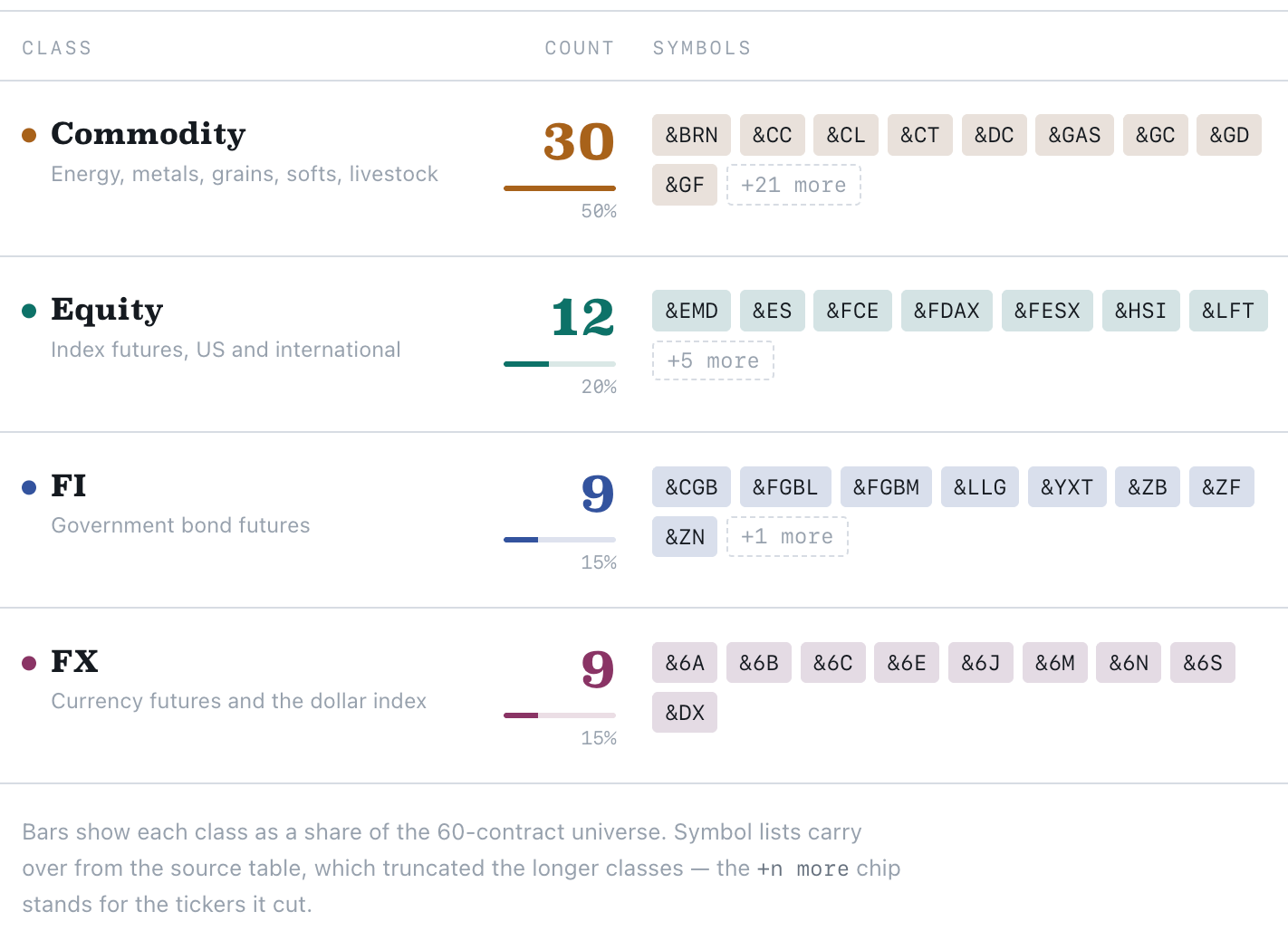
The paper uses 64 ratio-adjusted continuous futures from Pinnacle’s CLC database across four asset classes. We mirror it with 60 Norgate continuous futures.
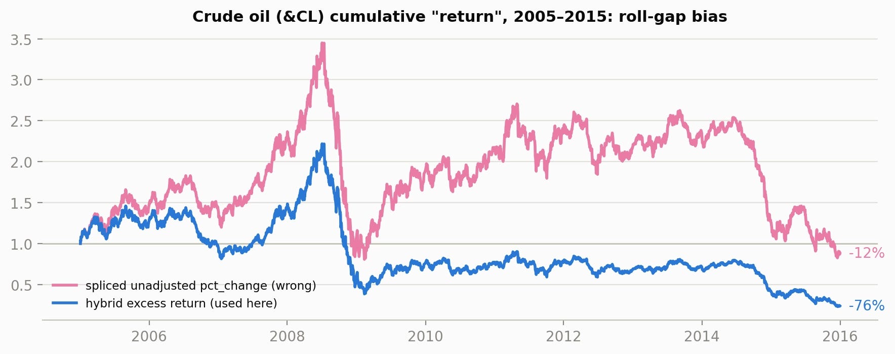
Norgate’s plain continuous symbol (e.g. &CL) is a spliced unadjusted series: at every roll it jumps from the expiring contract’s price to the next one’s without any P&L happening. Its pct_change is therefore not a return (for markets with steep carry the bias is enormous). The fix (standard in the futures literature, and equivalent to the paper’s ratio-adjusted data) combines both Norgate variants:
Features are computed on the synthetic ratio-adjusted index
The chart below shows what’s at stake for crude oil: the spliced series says -12% over 2005-2015; the true excess return was -76%.
B. Individual momentum features
Eight features per (date, asset), all from prices alone:
Vol-scaled returns over $\Delta \in \{1, 21, 63, 126, 252\}$ days:
Normalized MACD (Baz et al. 2015) for $(S,L) \in \{(8,24), (16,48), (32,96)\}$:
where $m(t,J)$ is a price EWMA with $\alpha = 1/J$. Every feature is winsorized at ±5 EWMA standard deviations (half-life 252).
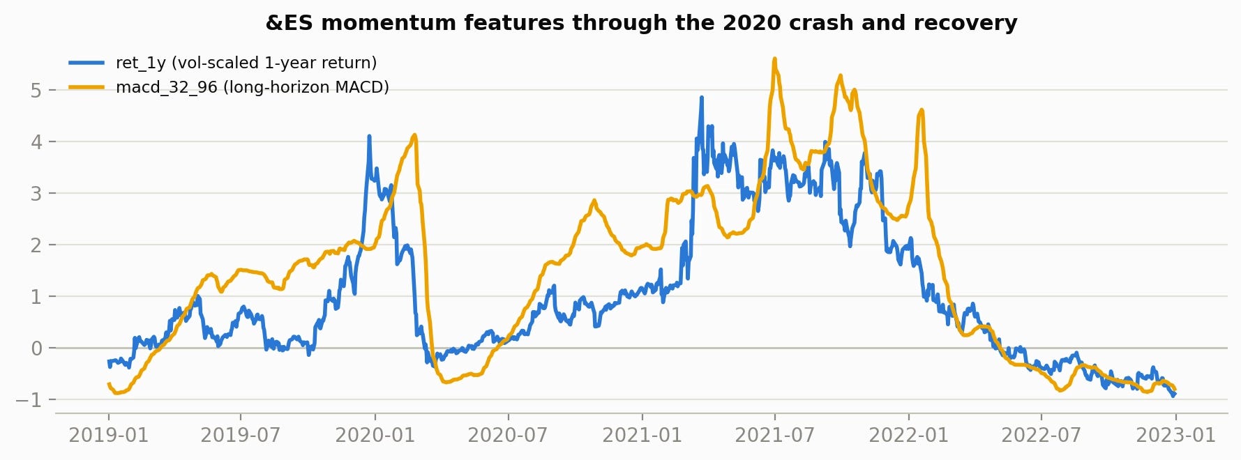
Here’s a sample of what we get:

C. Graph learning
This is the core of the paper. For each trading day $t$ and lookback $\delta$, stack each asset’s 8 features over the past $\delta$ days into $V_t \in \mathbb{R}^{N_t \times 8\delta}$ — each row is one asset’s momentum trajectory (for $\delta=1260$ that’s 10,080 columns). Only assets with complete windows qualify, so $N_t$ grows from ~33 (1990) to ~59.
The adjacency matrix solves the convex problem (Kalofolias 2016):

with $Z_{ij} = \|v_i - v_j\|^2$ (normalised by its mean so $\alpha,\beta$ are comparable across lookbacks).
Five graphs ($\delta \in \{252, 504, 756, 1008, 1260\}$) are averaged and degree-normalised:
Here’s the visualization of the learned graph for a given date:
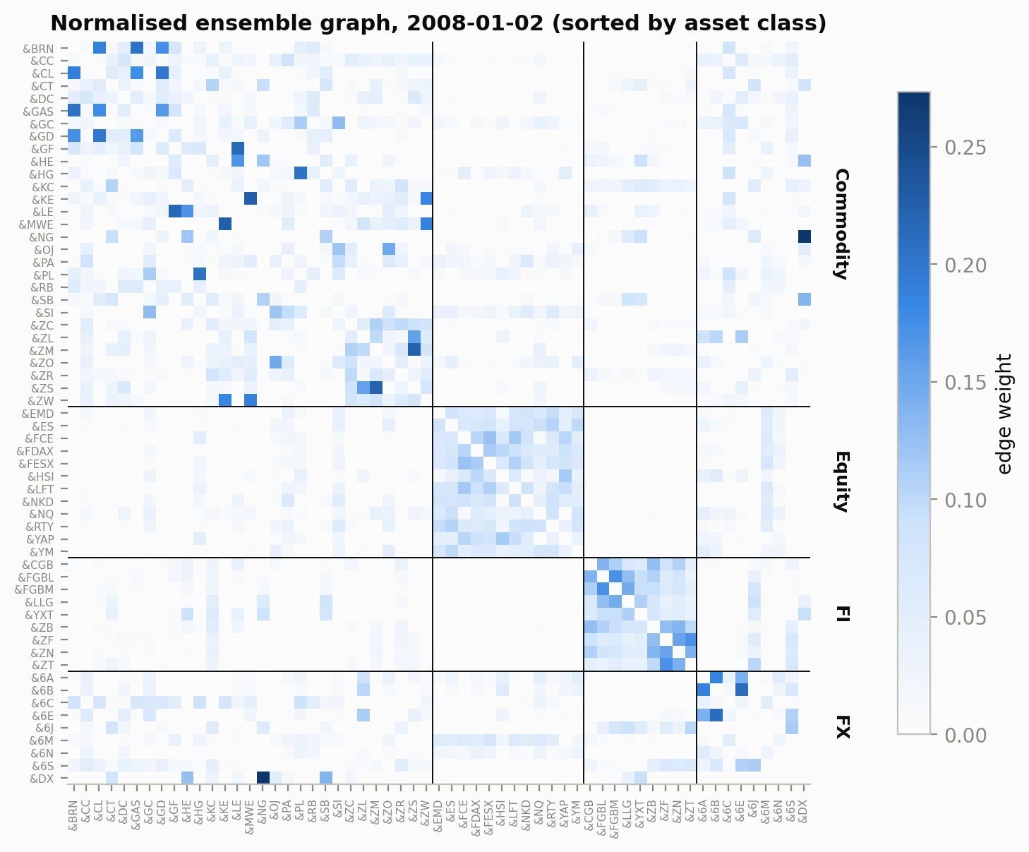
These are the top-3 edges of the ensemble graph on 2008-01-02 (α=1, β=0.3), learned purely from the similarity of momentum-feature trajectories, with no tickers, sectors, or asset-class labels supplied:
Wheat finds wheat. &ZW (CBOT soft red winter wheat) connects to &MWE (Minneapolis spring wheat) and &KE (Kansas City hard red winter wheat). The two other US wheat varieties, near-perfect substitutes trading largely on the same fundamentals, with soybean meal (&ZM) third, an adjacent CBOT feed-grain. The graph rediscovered the wheat complex from prices alone.
The US equity block assembles itself. &ES (S&P 500) links to &RTY, &YM, &NQ (Russell 2000, Dow, Nasdaq), i.e., all four US index futures cluster while European and Asian indices stay outside its top-3, capturing the region-level factor structure.
The Treasury curve clusters, with near-uniform weights. &ZN (10yr) connects to &ZF (5yr), &ZT (2yr), &ZB (30yr) at 0.15/0.14/0.14: the whole US duration complex, weighted almost equally, exactly what you’d expect for instruments driven by one yield curve.
Crude finds its physical and statistical relatives. &CL (WTI) links to &BRN (Brent) and &GAS (gasoil) (the same barrel and its refined product) plus &GD (S&P GSCI index), which is itself ~70% energy by construction, so the edge is essentially mechanical exposure the graph had no way of knowing about except through prices.
FX clusters by currency bloc. &6E (euro) picks &6B (sterling) and &6A (Aussie), co-movement against the common USD leg, plus a genuine inter-class edge to soybean oil (&ZL), plausibly the weak-dollar/commodity-boom co-trend of 2005-07 showing up in the momentum histories.
Precious metals + the dollar. &GC (gold) connects to &SI (silver) and &PL (platinum), then crosses asset classes to &6E: sensible, since gold and the euro share the anti-USD trade. These inter-class edges (gold↔euro, equity↔FX below) are precisely the connections the paper argues carry the incremental signal that individual momentum can’t see.
Asia-Pacific equities bridge to Europe. &HSI (Hang Seng) finds &YAP (Australian SPI 200) first (its regional partner), then &FDAX/&FESX, consistent with a global equity factor with a regional tilt.
Every neighborhood is economically legible (substitutes, curves, currency blocs, index overlap), yet the model was shown nothing but each contract’s own momentum history.
The economically sensible structure is an output, not an input.
D. Network momentum propagation
Each asset’s 8 network features are the edge-weighted average of its neighbors’ individual features (the asset itself is excluded, zero diagonal).
E. The regression
One pooled OLS across all assets and days: target $y_{i,t} = r_{i,t\to t+1} / \sigma_{i,t}$ . Models are refit every 5 years on expanding windows, features z-scored with training-window statistics only:
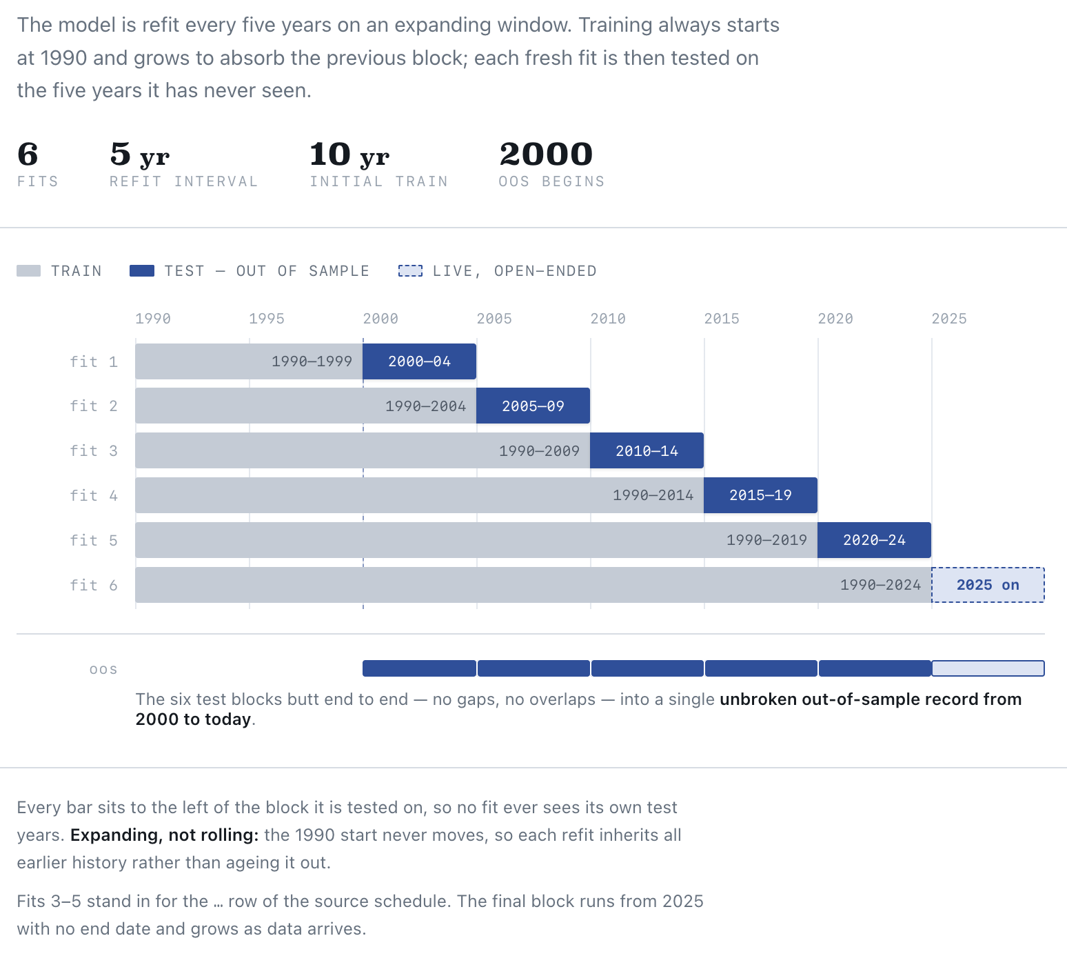
The standardized coefficients are a key replication checkpoint against the paper's Table 4: 1-day return positive, 1-month negative (short-term reversal), MACD(16,48) negative (mid-term reversal), with the reversal effects stronger in network momentum than individual momentum.
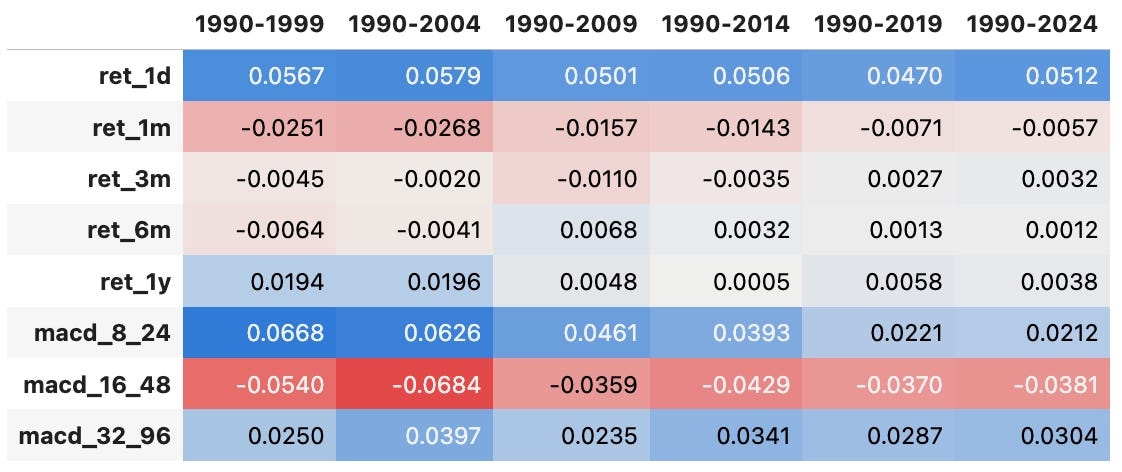
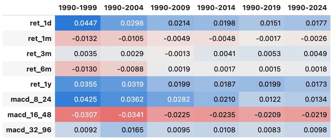
Both tables reproduce the paper’s pattern line for line: ret_1d positive everywhere, ret_1m negative (and roughly 2× stronger in GMOM than LinReg, the paper’s exact finding), the MACD +/−/+ signature across the three timescales, and all magnitudes decaying toward zero in later blocks as the anomalies weaken.
Now, let’s check the backtest.
Portfolio construction and backtest
Four strategies, all through the identical portfolio code (for the reference strategies we pass their signal as the “prediction”, so MACD uses the sign of the Baz $\phi$-rule rather than its continuous sizing):
Long Only: always +1 (the market benchmark)
MACD: model-free: $x = \tfrac13\sum_k \phi(y(S_k, L_k))$, $\phi(y) = y e^{-y^2/4}/0.89$
LinReg: the regression on the asset’s own features (no graph)
GMOM: the regression on network features
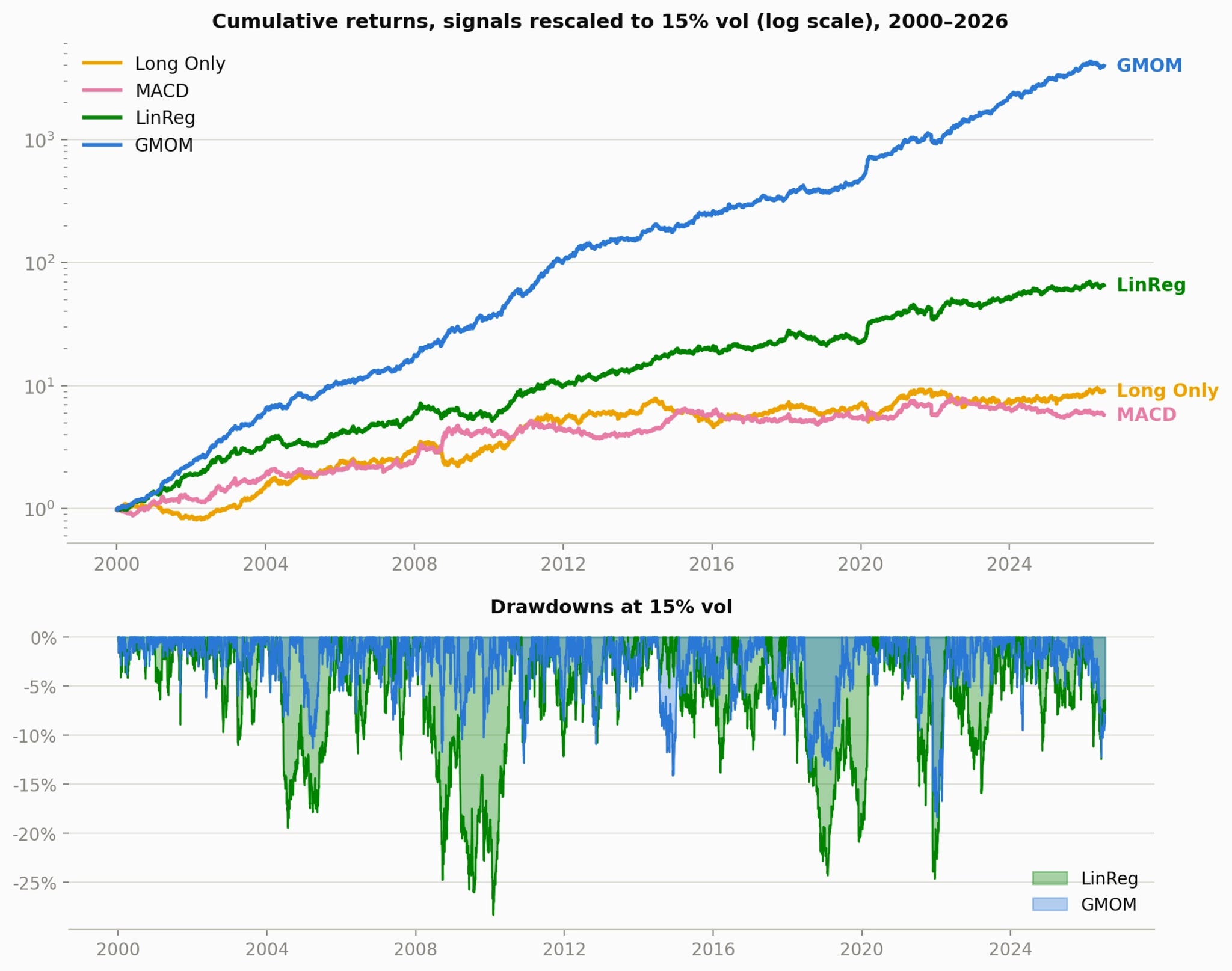
For comparability with the paper’s Panel B, each daily return series is rescaled to exactly 15% realized vol.
In summary:
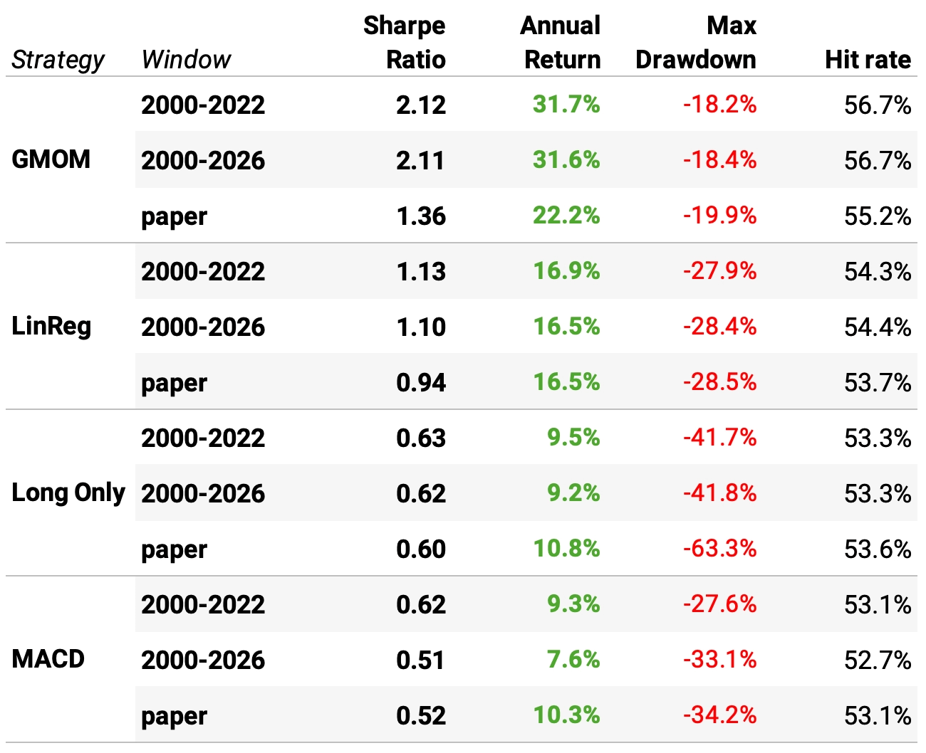
The paper’s ordering replicates exactly: GMOM > LinReg > Long Only ≈ MACD, with clear separation at every step. The graph adds ~+1.0 of raw Sharpe over the same regression run on the asset’s own features (2.11 vs 1.13): the network is doing the work, not the plumbing around it.
The three reference strategies land on top of the paper’s numbers (Long Only 0.63 vs 0.60, MACD 0.62 vs 0.52, LinReg 1.13 vs 0.94; returns and drawdowns at 15% vol within a few points). Since these share every pipeline component with GMOM except the graph, that closeness validates the data, features, and backtest end to end.
GMOM is also the best-behaved, not just the most profitable: smallest max drawdown of anything tested (-18% vs -28% LinReg, -42% Long Only at the same 15% vol) and the highest hit rate (56.7%).
The result is not fading out of sample of the paper: extending 2022 → 2026 leaves GMOM essentially unchanged (2.115 → 2.106) while the model-free MACD baseline decays (0.62 → 0.51).
Our GMOM exceeds the paper’s (2.10 vs 1.36), a gap large enough to warrant suspicion; this is why we ran a battery of diagnostics tests (in the next section: costs, hyperparameter luck, placebo graphs, regime concentration).
Why sharpe_raw: all Sharpes here are computed on raw, unscaled signals, gross of costs (the same basis as the paper’s Table 1 Panel A) so the comparison against their numbers is apples-to-apples. The return and drawdown columns are stated at a 15% vol target (their Panel B convention). We will analyze costs in the next section.
Let’s also look at daily return correlations:
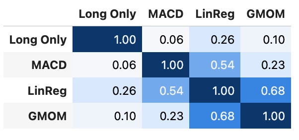
GMOM-LinReg correlation is 0.68, matching the paper’s ~0.65, despite identical input features. Only about half the variance is shared (0.68² ≈ 0.46): propagating momentum through the graph produces a genuinely distinct return stream, not a reweighted copy of individual momentum. Position signs agree ~73% of the time, again on top of the paper’s ~72%.
GMOM is nearly market-neutral (0.10 to Long Only). Its returns are essentially orthogonal to just holding the asset universe, so the Sharpe is coming from long/short timing, not embedded beta. LinReg carries more market exposure (0.26).
The graph pulls the signal away from classic trend-following. LinReg still co-moves with the model-free MACD baseline (0.54), while GMOM’s correlation to MACD drops to 0.23. Network momentum is the furthest of the three model strategies from a vanilla trend signal.
Diversification implication: with 0.68 correlation and both legs profitable, GMOM and LinReg combine usefully. This is consistent with the paper’s finding that RegCombo (both feature sets in one regression) edges out GMOM alone.
Diagnostics
A. Turnover and transaction costs
Our GMOM exceeds the paper’s. Let’s run diagnostic tests to thoroughly verify the results. We will run 4 independent ways to double-check them, starting with turnover and transaction costs:
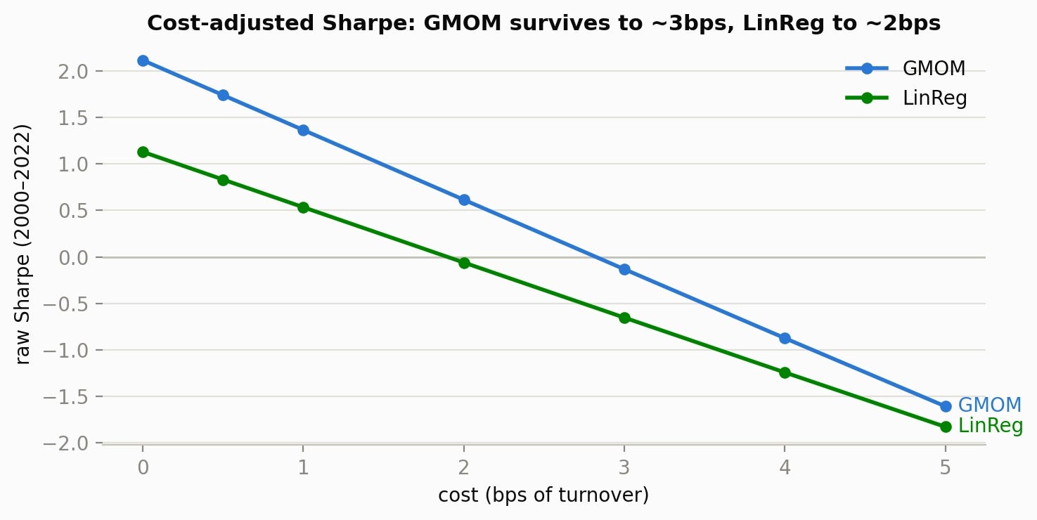
Highlights:
Costs are charged per unit of turnover: each strategy pays c bps on daily position changes, sweeping c = 0-5bps. The headline numbers are the c = 0 column; the full table is in the code notebook.
At realistic costs for futures this liquid (0.5–1bp), GMOM nets Sharpe 1.74-1.37, still above the paper’s gross 1.36, while LinReg drops to 0.83-0.53.
Cost-resilience ordering replicates the paper: GMOM stays positive to ~3bps, LinReg only to ~2bps. The network signal buys roughly an extra basis point of cost headroom at every level.
The honest caveat is turnover: GMOM trades 1.46 σ-scaled units/day (vs 1.00 for LinReg, and ~0.5 in the paper). Per unit of gross alpha we churn harder than the paper: the signal is fast, flipping signs frequently.
That churn is addressable: signal smoothing is the paper’s own top future-work suggestion, and with 2.1 gross Sharpe there is ample room to trade alpha for cost room. We implemented that, it’s our last section (a 2-day EWM cuts turnover ~30% for only ~0.13 of gross Sharpe).
B. Hyperparameter sensitivity: Is 2.1 a lucky spike?
The graph depends on the choices for alpha and beta (their product). Sweeping 5 products, here’s what we found:
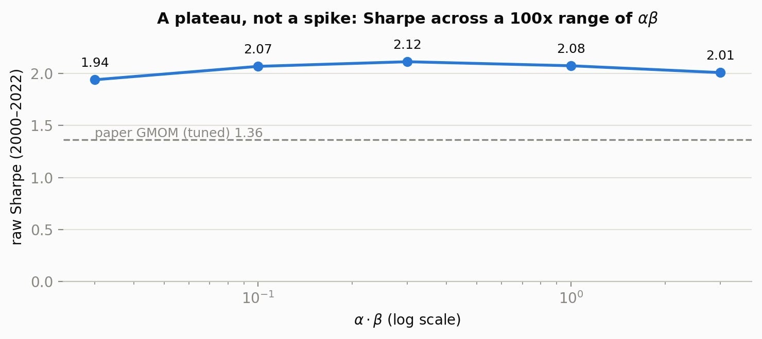
One sweep covers the paper’s entire 11×11 grid: the degree-normalized graph depends on α and β only through their product, so the 1-D sweep over a 100× range of αβ spans everything the paper tuned over, from sparse graphs (~6 neighbors per asset) to nearly complete ones (density ~0.93).
The result is a plateau, not a spike: raw Sharpe moves only 1.94 → 2.12 → 2.01 across that whole range, and every single untuned point clears the paper’s tuned GMOM (1.36). The excess over the paper cannot be hyperparameter luck: there is essentially nothing here to overfit.
C. Placebo graphs: Is the learned structure doing anything?
If GMOM’s edge survived information-free graphs, it would just be a clever way of smoothing cross-sectional momentum. Let’s check 2 placebos: a uniform graph (network feature = cross-sectional mean excluding self) and random Erdős-Rényi graphs at the ensemble’s density, both degree-normalized identically and run through the identical regression pipeline.
Here are the results:
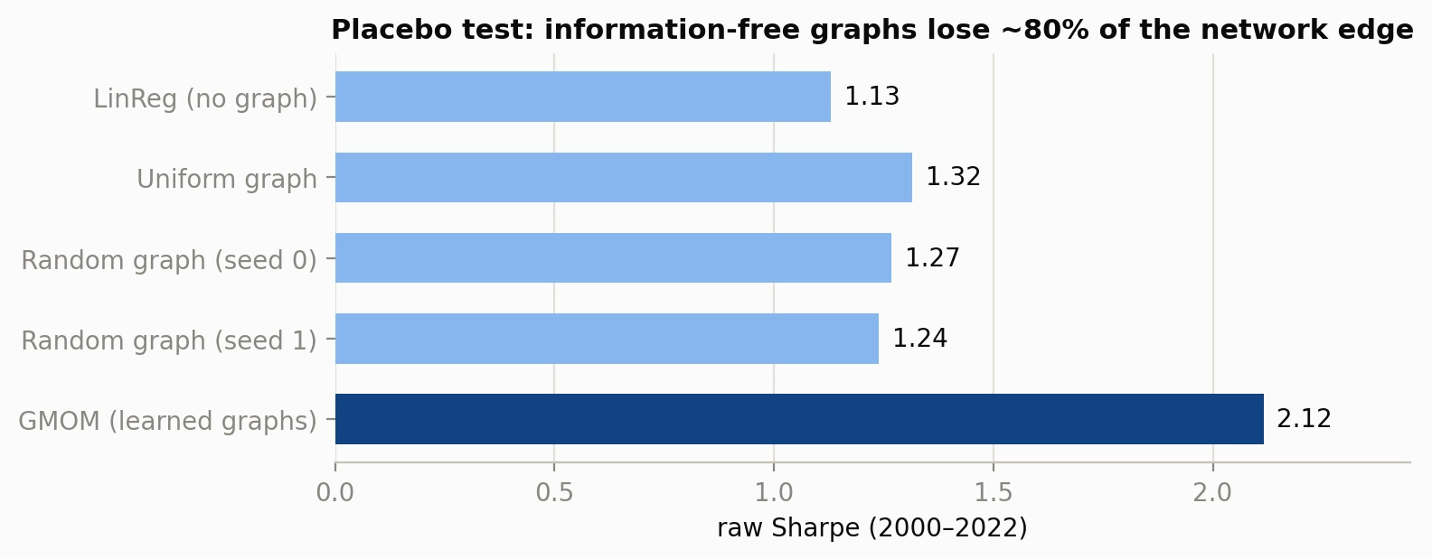
The highlights are striking:
Information-free graphs lose ~80% of the network edge. Replacing the learned graphs with a uniform graph (cross-sectional mean of everyone else) or random Erdős-Rényi graphs at the same density (run through the otherwise identical pipeline) collapses Sharpe from 2.12 to 1.24-1.32. Graph mechanics (any averaging) is worth ~+0.2 over LinReg’s 1.13; the learned similarity structure adds the other ~+0.8.
The placebos aren’t just weaker, they’re riskier: worst drawdowns of anything tested (-32/-36% at 15% vol), because averaging over the wrong neighbors smears bad signals across the whole book. GMOM’s edge is genuinely the learned structure, not a smoothing artifact.
D. Regime robustness: Is the edge concentrated in one era?
Here are the annual results:
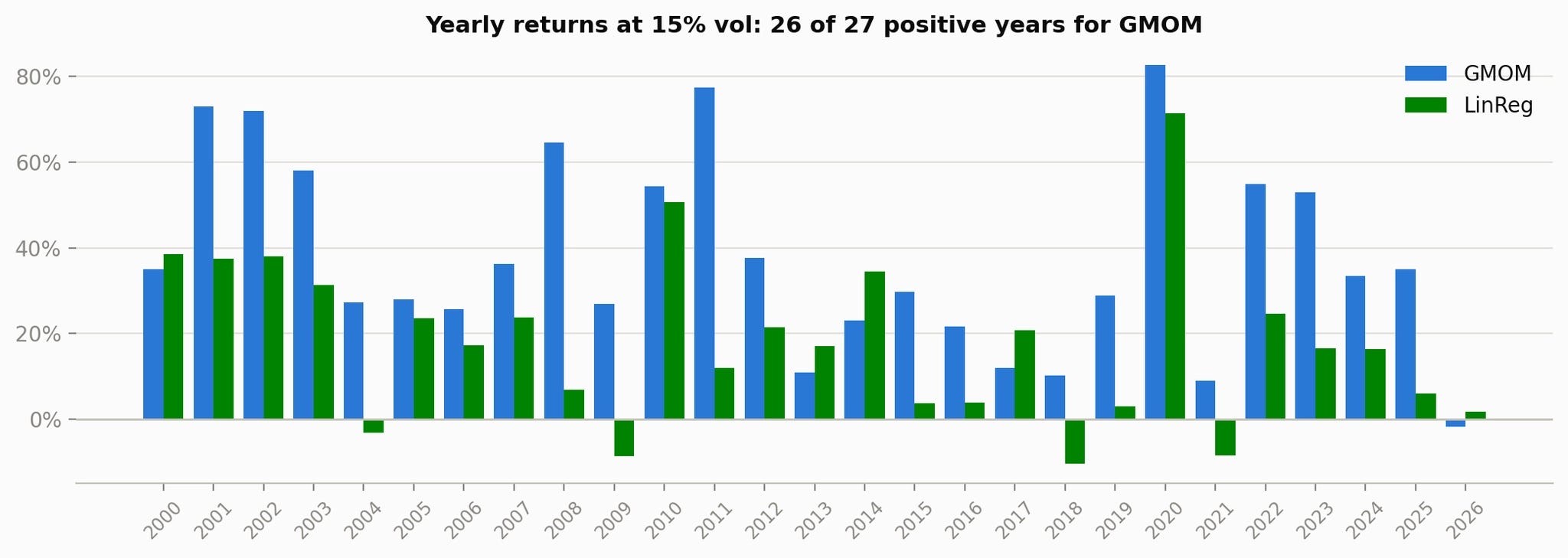
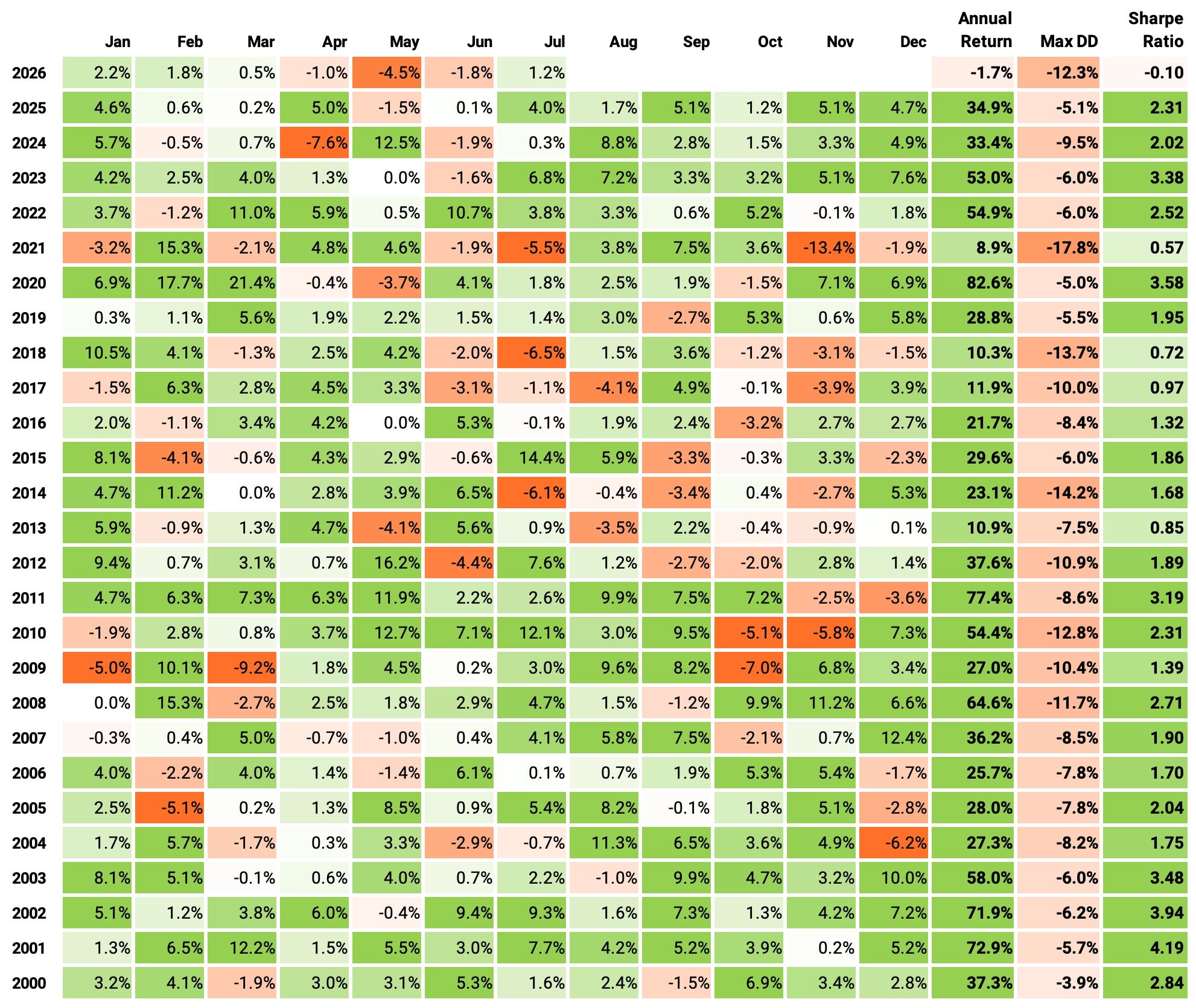
The edge is broad, not episodic: 26 of 27 years positive at 15% vol (the sole exception is the partial 2026, roughly flat), versus five losing years for LinReg. No single era carries the result.
Crisis convexity, amplified: the biggest years are exactly the trend-following crises: the dot-com unwind (2001–03), +65% in 2008, 2011, +85% in 2020, 2022. The weakest stretch is the 2013-2018 “momentum winter”, where GMOM grinds out small positive years while LinReg loses money.
But there’s a decay: first-half Sharpe 2.46 vs second-half 1.73: the softening is real, but even the recent-decade figure still exceeds the paper’s tuned full-sample number.
Let’s see now how can we improve the high-turnover.
Signal smoothing
As we saw previously, the strategy churns 1.46 units/day. This is the flip side of a fast signal. The paper’s own top future-work item is turnover regularization.
The simplest version is smoothing the prediction with a per-symbol EWM before signing it:
Positions then flip only when the smoothed prediction changes sign, not on every day-to-day wobble. The sweep below compares spans 1 (no smoothing) through 21 on gross Sharpe, turnover, and net Sharpe at each cost level:
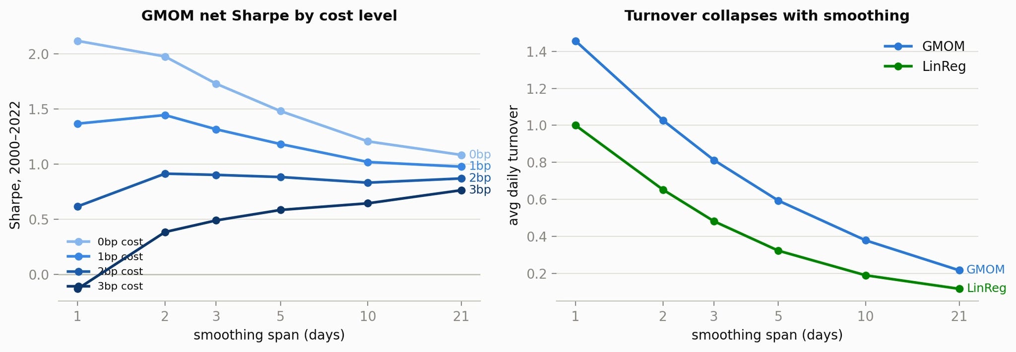
Highlights from the sweep:
Span 2 is close to a free lunch: turnover falls 30% (1.46 → 1.03) for only 0.13 of gross Sharpe (2.10 → 1.97), and it dominates the unsmoothed strategy at every cost level ≥ 1bp: at 2bp it holds Sharpe 0.91 vs 0.60, at 3bp it stays positive (+0.38) where unsmoothed goes negative. Breakeven cost moves from ~2.9bp to ~3.5bp, and MDD even improves slightly. Recommended default: span 2 (span 3 if trading nearer 2-3bp).
The cost regime picks the span: at ≤0.5bp smoothing is a wash; only above 3bp do long spans (10-21) win, and at those costs this daily strategy shouldn’t be traded at all.
The alpha is fast. GMOM’s gross Sharpe halves (2.10 → 1.08) as the span stretches to a month, while LinReg only drops 1.12 → 0.83. The network signal decays faster than the individual one. Propagation is capturing short-lived cross-asset lead-lag effects (consistent with the regression’s largest weight on the 1-day feature), not slow trend. That is also why unsmoothed GMOM churns 46% more than LinReg: fast signals cross zero often. We can smooth away the cost problem, but not into a slow strategy: the edge lives at the 1-3 day horizon.
But isn't that just timezone lookahead bias?
After publication, a reader of the published piece raised this:
“Have you tried removing non-US futures that trade in a different time zone? In my replication that reduced Sharpe to 0.7, meaning there is a lookahead bias from one timezone to another.”
So, in this new section (written after the initial publication) we will test that claim on our replication, in 4 steps:
Universe split: which of our 60 instruments settle outside US hours;
P&L decomposition: where the published GMOM Sharpe actually comes from, US vs non-US legs;
Mechanistic check: do same-date US closes “predict” next-date non-US closes far more than the reverse;
Clean rerun: re-learn every graph and regression on a US-session-only universe.
The mechanism being tested
The pipeline treats all of date ‘s closes as simultaneous. They are not. Eurex/ICE-Europe settle ~5-6 hours before the US close; Hong Kong and Sydney settle ~12-15 hours before it. So a non-US asset’s “date “ feature row is stale by the time US markets close, and (this is the harmful direction) a signal formed for a non-US asset at date uses US features observed hours after that asset’s date- close. The backtest then books the non-US close-to-close return , part of which has already elapsed when the US information arrives. Any genuine US→overnight-Asia/Europe spillover is partially untradable at those closes: in daily close data it shows up as free predictability.
Propagation through the graph is exactly a cross-asset average, so GMOM is maximally exposed; LinReg (each asset’s own features only) has no cross-asset channel and serves as the control.
Let's get started:
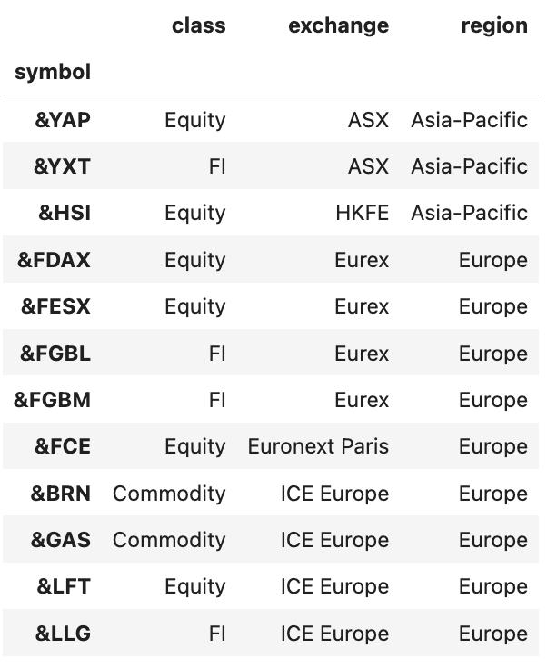
1. Which instruments settle outside US hours
Exchange per Norgate metadata. Two deliberate keeps:
&NKD(Nikkei 225) stays US: the underlying is Japanese but the contract trades and settles on CME in Chicago hours.&CGB(Canadian 10yr) stays US-session: the Montreal Exchange runs on Eastern time and closes alongside the US session. No timezone gap, even though it is technically non-US.
That leaves 12 different-timezone instruments out of 60, the set a US-close-anchored daily bar cannot treat as simultaneous:
2. Where the published Sharpe comes from: P&L decomposition
Same cached full-universe run as the article (graphs, regressions, predictions all untouched). We only split the daily portfolio average into the legs traded on US-session symbols vs the 12 different-timezone symbols, for GMOM and for the LinReg control:
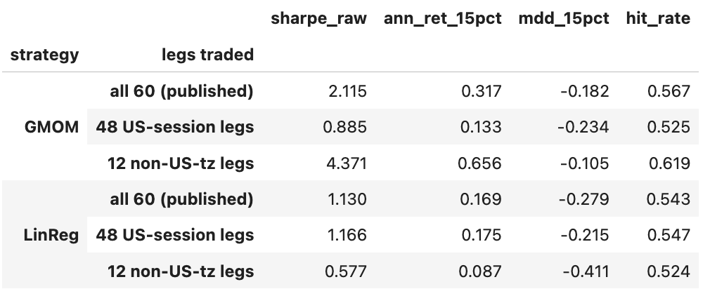
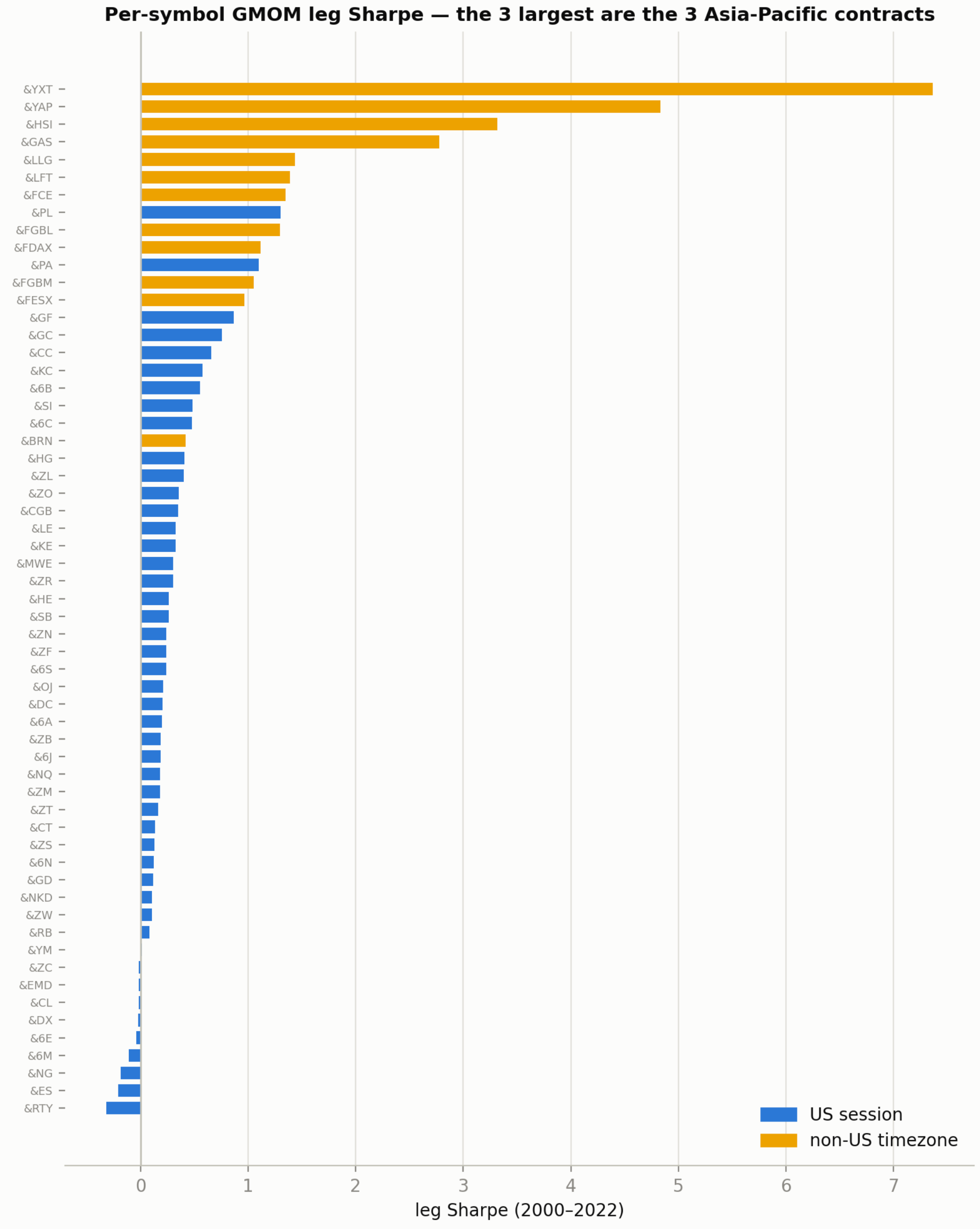
The signature is unmistakable. GMOM's 12 non-US legs run a 4.4 Sharpe on their own while its 48 US legs manage 0.88. A fifth of the headline 2.12 comes from four-fifths of the book, and the tiny non-US sleeve carries the rest. LinReg, fed the same per-asset information but with no cross-asset channel, shows the opposite pattern (US 1.17, non-US 0.58): the non-US markets are not intrinsically easier… they only become "easy" when same-date cross-asset information flows through the graph. The 0.88 US-legs figure also lands right where the commenter's US-only replication did (~0.7).
3. Mechanistic check: the lead-lag is one-directional
If the graph were harvesting a real, tradable cross-asset effect, predictability should not care about closing-time order. If it is harvesting the timezone gap, today’s US closes should “predict” tomorrow’s non-US closes (whose intervals overlap the US close) far better than non-US closes predict tomorrow’s US closes, and far better than US predicts US.
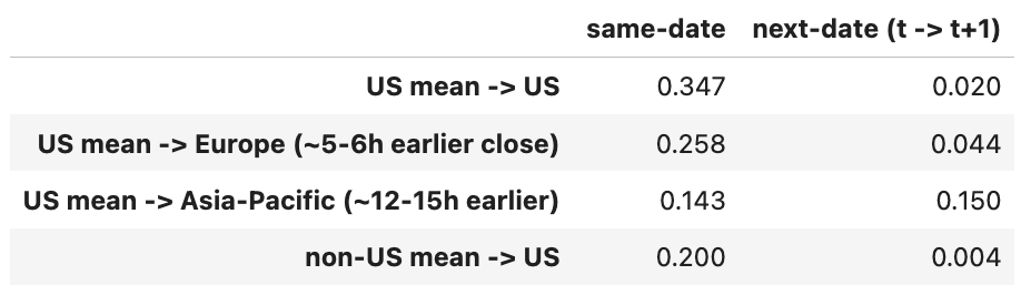
Predictability follows the clock, not the economics. Same-date correlations are similar in both directions (~0.2 each way, global markets co-move). But at one-day lag the symmetry breaks: today's US mean "predicts" tomorrow's non-US closes at +0.07 average correlation, versus +0.004 for the reverse direction and +0.02 for US→US. And within the non-US group the effect is monotone in the size of the timezone gap: +0.044 for Europe (5–6h overlap), +0.15 for Asia-Pacific (12–15h). A real momentum-spillover effect has no reason to care which market's clock closes first, let alone scale with the number of overlap hours. A close-timestamp artifact has to. The tell inside the table: for Asia-Pacific the next-date correlation (+0.15) exceeds the same-date one (+0.14), because a Sydney or Hong Kong "tomorrow" close is nearer in wall-clock time to today's US close than its own "today" close is. This is also why &YXT, &YAP and &HSI post the absurd 3.3–7.4 leg Sharpes above: an Asian "next-day" close is mostly a delayed echo of information the US close already printed.
4. The clean test: US-session-only universe, end to end
Drop the 12 different-timezone instruments before anything is computed: features, graph learning (all 5 lookbacks, every date), propagation, and the expanding-window regressions all see only the 48 US-session instruments. Same hyperparameters as published. LinReg gets the identical treatment as the control.
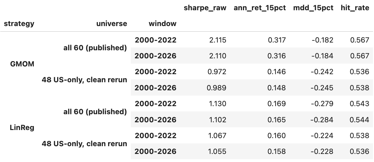
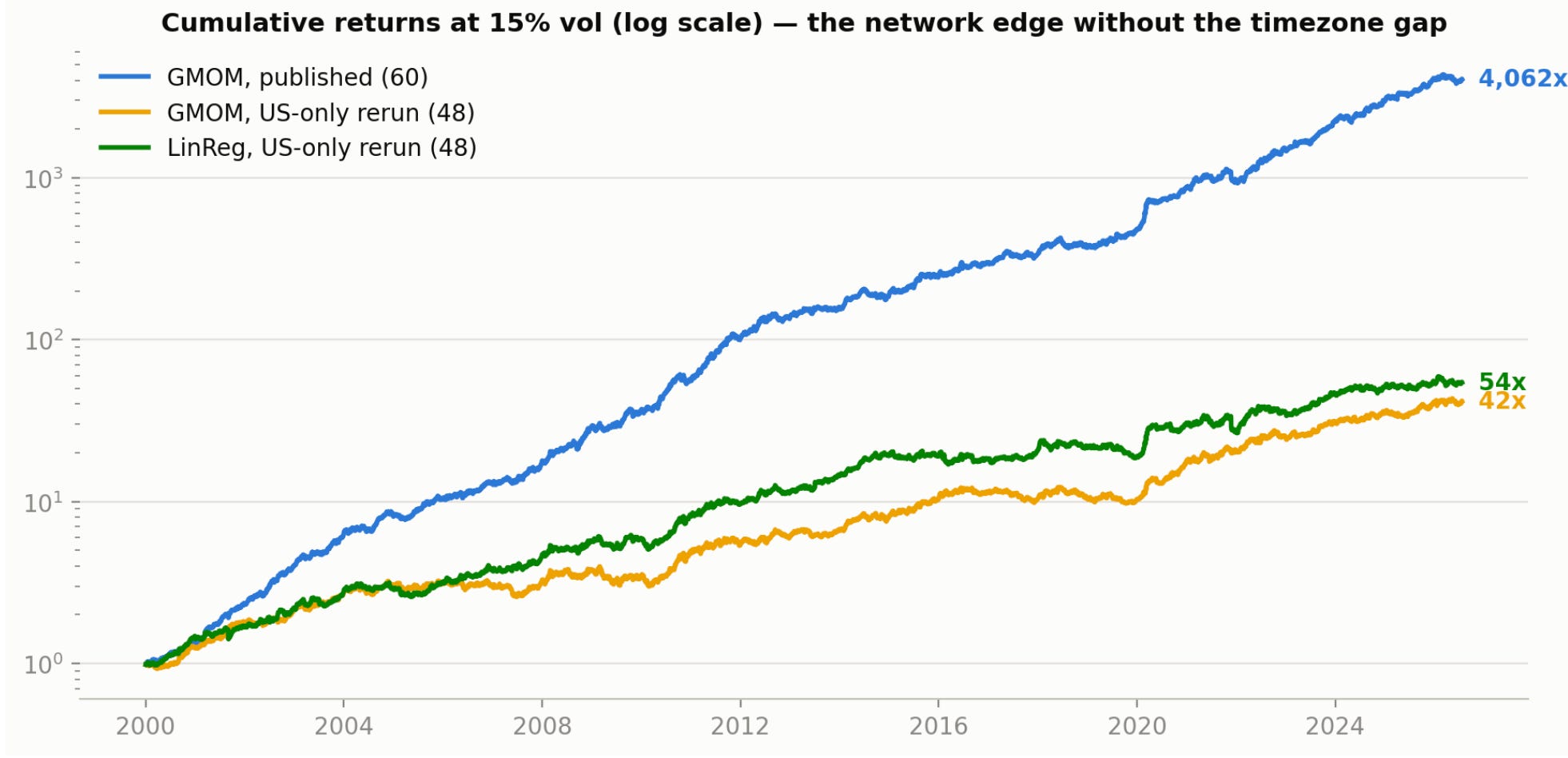
The comment is right. The network momentum edge in our replication is timezone lookahead:
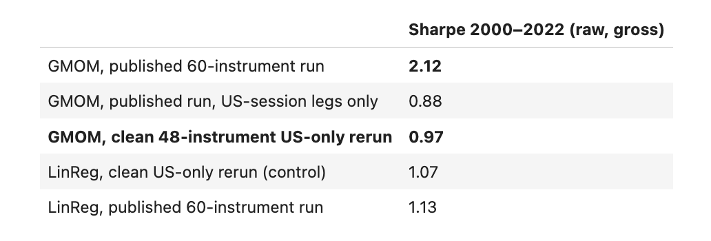
The headline collapses from 2.12 to 0.97 when the 12 different-timezone instruments are removed before anything is computed, right in line with the commenter’s ~0.7 (residual difference is universe composition). Our published number was inflated ~2.2×.
The graph adds nothing once closes are synchronous. Clean GMOM (0.97) lands at or slightly below the clean LinReg control (1.07). The entire +1.0-Sharpe “network premium” we attributed to learned graph structure was the graph harvesting the US-close → earlier-close-market lead-lag, which is unexploitable at the closes the backtest assumes. LinReg, with no cross-asset channel, is untouched by the ablation (1.13 → 1.07), the bias lived precisely and only in the propagation step.
Every diagnostic in the article now reads differently, coherently. The regression’s dominant
ret_1dweight, the alpha that halves under a one-month smoothing (”the edge lives at the 1-3 day horizon”), and even the placebo graphs retaining Sharpe 1.24–1.32 (uniform/random graphs also propagate same-date cross-asset information, so they were contaminated too): all are signatures of a one-day timezone artifact, not of momentum spillover. The battery of diagnostics we ran (costs, hyperparameter sensitivity, placebos, regime breakdown) could not catch this class of bug, because every variant shared the same asynchronous-close data.The paper itself is exposed to the same mechanism. The Pinnacle universe includes DAX, CAC, FTSE, Hang Seng, SPI, Australian bonds, gilts, bunds. We cannot rerun their exact data, but there is no reason the bias spares them; their more modest GMOM-over-LinReg gap (1.36 vs 0.94) is consistent with the same artifact at smaller magnitude.
What a legitimate test of network momentum would need: synchronous prices (e.g. sample every instrument at one common timestamp from intraday data), or an execution-honest backtest that only lets a non-US position use information available before that market’s own close (lag non-US signals by one day, which hands the artifact zero credit but also destroys any genuine intraday spillover), or simply a single-session universe, as here.
Final thoughts
So, does network momentum hold up? Our first version of this article said: emphatically, yes. We now owe you a correction: no, not in daily close data. And we owe the correction to a sharp-eyed reader.
After publication, Maxim Edelman asked a deceptively simple question: had we tried removing the non-US futures that trade in a different time zone? In his replication, that alone cut the Sharpe to 0.7, suggesting the edge was lookahead bias leaking from one timezone to another. We ran the test. He’s right, and we’re grateful he pushed us to look.
Here’s what the ablation found:
The alpha lives exactly where the clock is broken. Twelve of our 60 instruments settle hours before the US close (nine European, three Asia-Pacific). Those 12 legs alone run a 4.4 Sharpe in the published GMOM; the 48 US-session legs manage 0.88. LinReg (same information, no cross-asset channel) shows the opposite pattern. The bias lives precisely and only in the graph’s propagation step.
Predictability follows the clock, not the economics. Today’s US market mean “predicts” tomorrow’s non-US closes at +0.07 correlation, versus +0.004 in the reverse direction, and the effect scales with the timezone gap (Europe +0.04, Asia-Pacific +0.15). The per-symbol leg Sharpes are a caricature of this gradient: the three Asia-Pacific contracts post 3.3, 4.8, and 7.4. A real spillover effect has no reason to care which market closes first. A timestamp artifact has to.
The clean rerun settles it. Re-learning every graph and regression on the 48 US-session instruments: GMOM drops from 2.10 to 0.97, at or slightly below the 1.07 LinReg control. Once closes are synchronous, the network adds nothing.
The uncomfortable lesson is that our four-angle diagnostics battery (costs, hyperparameter sweeps, placebo graphs, regime breakdowns) never stood a chance, because every variant shared the same asynchronous-close data. The placebo test we were proudest of was itself contaminated: uniform and random graphs also propagate same-date cross-asset information, which is why they retained a 1.2-1.3 Sharpe. In hindsight, the artifact was hiding in plain sight in our own findings: the regression’s dominant 1-day feature, the alpha that halved under a month of smoothing, our conclusion that “the edge lives at the 1-3 day horizon.” It does, because that’s the horizon at which the timezone gap operates. And since the paper’s own Pinnacle universe contains the same DAX, CAC, FTSE, Hang Seng, SPI, gilt and bund contracts, we suspect its more modest GMOM-over-LinReg gap (1.36 vs 0.94) carries the same bias at smaller magnitude.
What survives? The pipeline replication stands: the excess-return methodology, the features, the graph learner, the reference strategies landing on the paper’s numbers. Plain individual momentum survives untouched at ~1.1. Even the most satisfying finding survives as structure: fed nothing but momentum histories, the graphs really do rediscover the wheat complex, the Treasury curve, and the gold-euro anti-dollar trade. But economically sensible structure, it turns out, does not equal tradable alpha: not when the backtest treats a 4pm Chicago close and a 4pm Hong Kong close as the same instant.
Is the work done? Differently than we thought:
Test network momentum honestly: synchronous prices (sampling every instrument at one common intraday timestamp), or signals that only use information available before each market’s own close. That test is still worth running, genuine overnight spillover may exist; it just can’t be harvested at closes that already happened.
Treat “too good” as a bug report. We wrote that a 2.10-vs-1.36 gap “made us suspicious,” then let a battery of same-data diagnostics reassure us. We forgot to look into the data. Garbage in, garbage out.
Publish anyway. Four diagnostics of ours missed what another research caught. That’s not an argument against sharing results, it’s the whole argument for it.
Barabási was right that networks are everywhere. But what our graph learner found in this pile of futures prices wasn’t momentum quietly propagating from asset to asset… it was the rotation of the Earth. Thank you, Maxim, for having the eye we lacked.
As always, I’d love to hear your thoughts. Feel free to reach out via Twitter or email if you have questions, ideas, or feedback.
Cheers!
PS: That's why peer review is so important to science… Nullius in verba ;)
Have you tried removing non-US futures that trade in a different time zone? In my replication that reduced Sharpe to 0.7 meaning there is a lookahead bias from one timezone to another.