Portfolio Optimization
Coding Mean-Variance Optimization to +1.7 Sharpe


The idea
“An investor who knew future returns with certainty would invest in only one security.” — Harry Markowitz
We don’t know the future. This is why we intuitively spread our bets. Harry Markowitz turned that intuition into algebra. In 1952, he published a paper that gave diversification a rigorous mathematical foundation, proving not just that it works, but exactly how much of each asset to hold given your tolerance for risk. The Nobel committee caught up with him in 1990. His Nobel lecture is worth reading.
The idea for this article came to me while I was reading a new paper titled “Diffusion Factor Models.” The paper addresses one of the main problems of naive Mean-Variance Optimization: estimation error arising from unreliable sample means and covariances when the number of assets exceeds the number of available observations.
The authors’ proposed solution is elegant. Rather than directly estimating moments from limited data, they train a diffusion model that learns the underlying factor structure of asset returns, then generate abundant synthetic samples to obtain more stable estimates. This approach effectively trades a small modeling bias for a substantial reduction in estimation variance, achieving Sharpe ratios nearly three times higher than equal-weight benchmarks (1.36 vs. 0.49) and dramatically outperforming traditional shrinkage methods, which produced negative returns in the same test period.
In fact, the paper provides direct evidence of an important insight in portfolio optimization: accurate covariance estimation matters more than accurate mean estimation for portfolio performance. Their hybrid methods reveal this clearly: combining naive sample means with diffusion-generated covariances achieves a Sharpe ratio of 1.09, while the reverse — diffusion-generated means with naive sample covariances — yields only 0.28.
But I’m not writing about that paper this week. I’m going to test their method first, then come back to it later this year. This week is about classic Mean-Variance Optimization. We have to crawl before we walk.
Our problem is simpler: allocating capital across a handful of substrategies rather than hundreds of individual assets. In our setting, estimating means and covariances won’t be a problem; we’ll have far more observations than parameters to estimate.
Here’s the plan:
First, we’ll introduce the set of strategies we want to combine.
Next, we’ll establish a baseline using an equal-weight allocation.
Then, we’ll implement mean-variance optimization in Python.
Finally, we’ll evaluate the results and outline the next steps.
We’re building a private community for systematic traders. A place to explore ideas, exchange insights, and tackle the real technical and strategic challenges of building robust trading systems… from signal research to execution and risk.
Enrollment reopens at the end of this month. Join the waitlist below to be the first to know when new seats open:
Speaking of great reads, there’s a new Substack I’d recommend:

I’ve found several of his articles genuinely insightful. Hope you enjoy them as much as I do.
The portfolio we’re actually optimizing
In our last article (Murphy’s Law), we stress-tested a simple mean-reversion system and treated “anything that can go wrong will go wrong” as a design principle: assume failure modes exist, then engineer around them. Here’s the summary of what we did:
Base strategy (mean reversion in liquid equities): when a stock suffers a statistically extreme short-term drop, we buy the dislocation (with simple regime filters like “in an uptrend” and a low short-term QPI), then hold briefly for the rebound.
Better entry timing: instead of waiting for the next open, we test entering at the close to capture the earliest part of the rebound and reduce “gap risk” around the entry.
Signal refinements: we progressively tighten what qualifies as a “good” dislocation (stronger/cleaner setups, better regime constraints, fewer low-quality events).
Walk-forward research loop: parameters are selected out-of-sample via rolling walk-forward tests (train → validate → deploy), rather than tuned once on the full history.
Ensemble mindset: instead of betting on one “best” parameter set, we combine a small basket of strong variants to reduce overfitting and smooth performance.
Different universes
An easy way to diversify this kind of system is to run the same playbook in other markets. Let’s see how it behaves across three universes:
US: S&P 500 constituents (last week’s setup, max of 10 positions)
Canada: S&P/TSX Composite constituents (max of 5 positions)
Australia: S&P/ASX 200 constituents (max of 5 positions)
In summary:
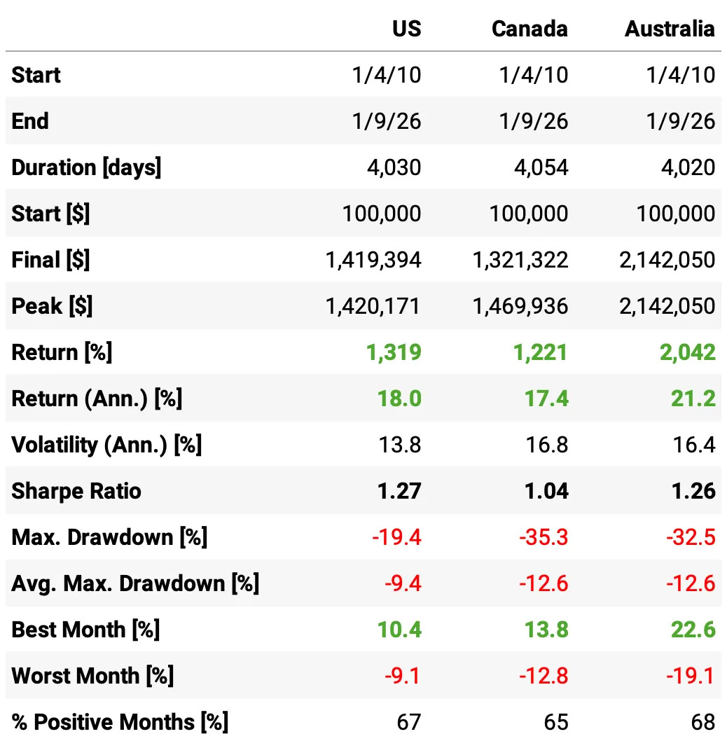
The approach works in all three markets: ~17–21% annualized returns with ~1.0–1.3 Sharpe across US/Canada/Australia (since 2010).
The trade-off: outside the US we earn comparable performance, but with materially deeper drawdowns (~-33% to -35% vs -19% in the US).
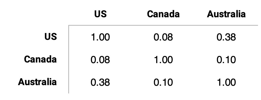
Diversification benefits will be strong: cross-geo correlations are very low — US-Canada 0.08, Canada-Australia 0.10, and even the highest pair (US-Australia) is only 0.38.
I’m starting the tests in 2010 (instead of 2003) because the strategy is extremely profitable pre-2010 in Canada and Australia, and I don’t want the results to be dominated by that unusual period.
Baseline: equal-weight portfolio
Now let’s see what happens with the naive approach: equal weights across strategies, rebalanced annually:
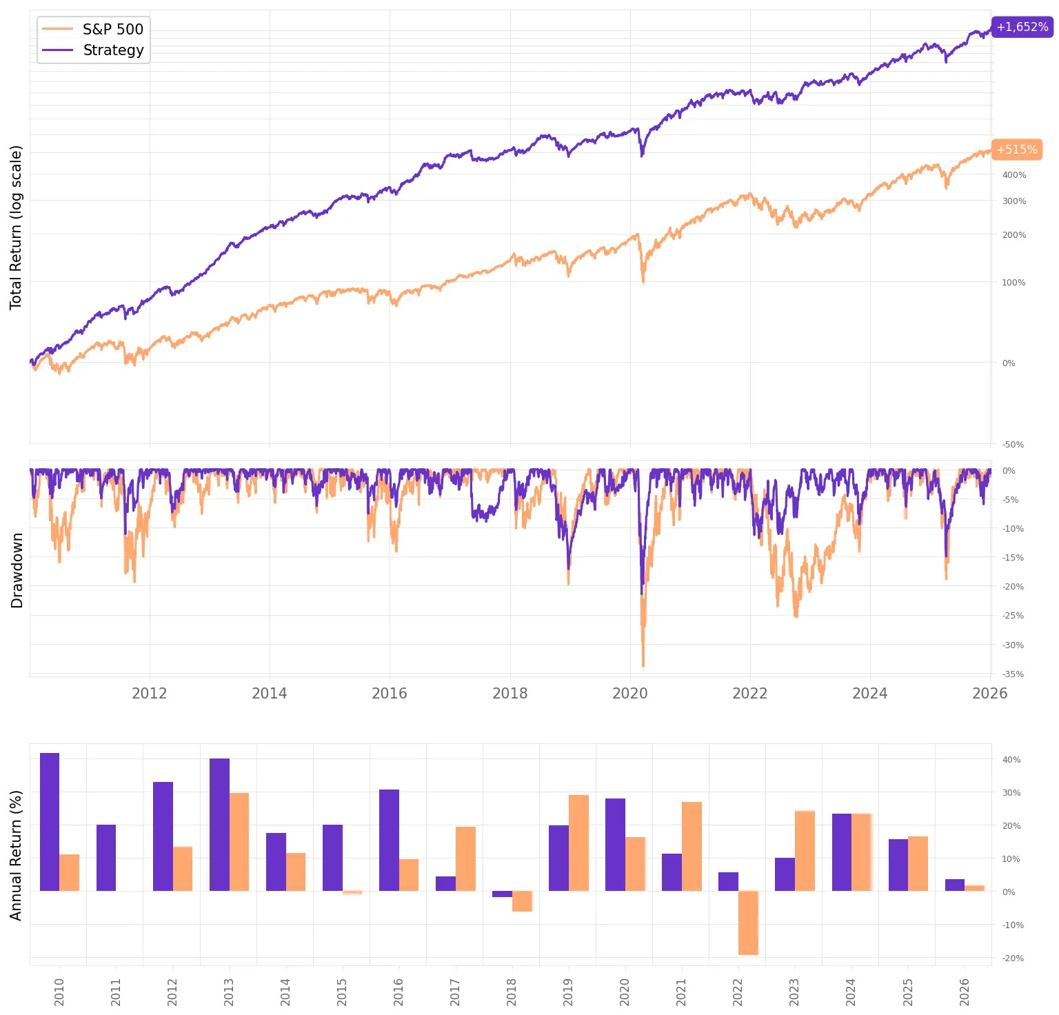
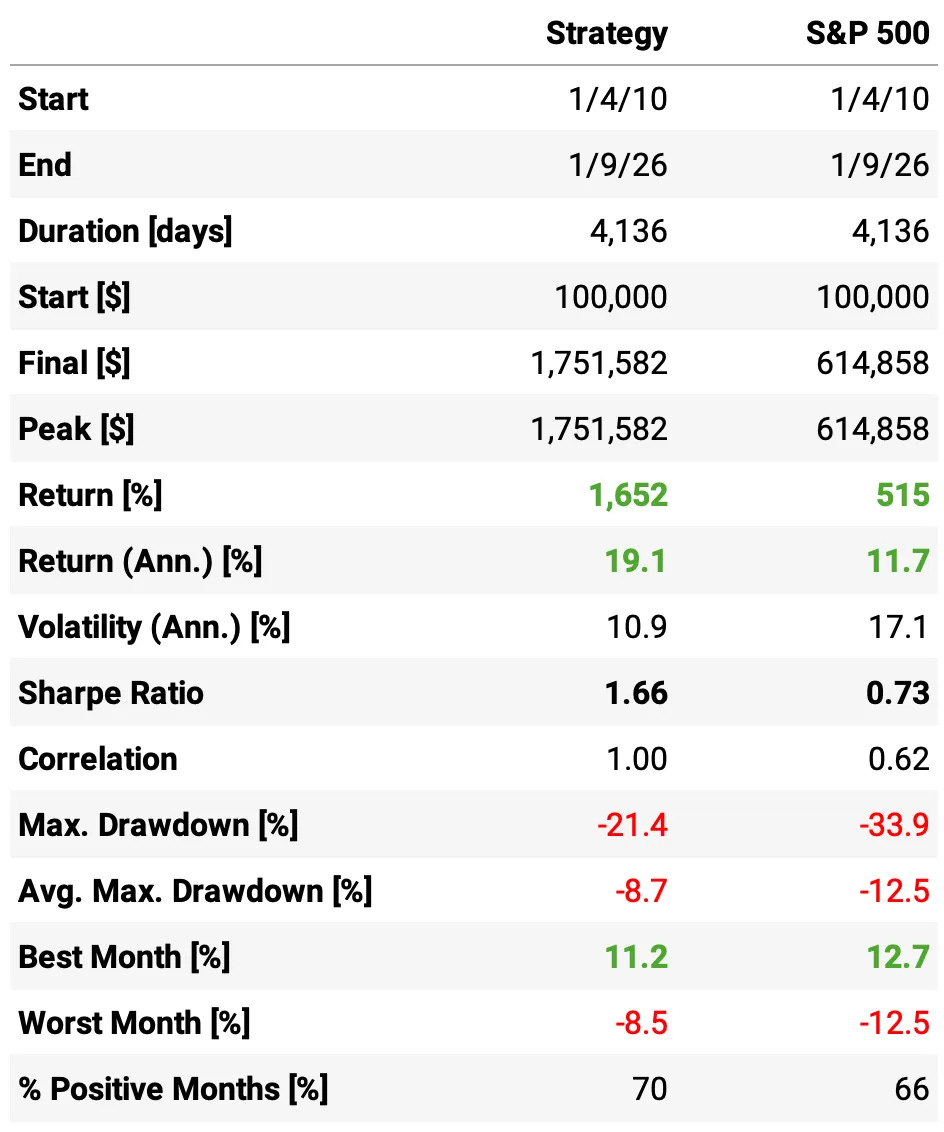
Volatility collapses with diversification: the equal-weight portfolio runs at 10.9% vol, versus 13.8% (US), 16.8% (Canada), and 16.4% (Australia). This is a big drop in risk despite holding three “risky” sleeves.
Sharpe jumps meaningfully: 1.66 for the equal-weight portfolio vs 1.27 (US), 1.04 (Canada), 1.26 (Australia). “Same-ish returns, much lower variance” effect.
Returns stay high while risk falls: annualized return is 19.1%, right in the middle of the single-country range (17.4%-21.2%), but achieved with far less volatility.
Drawdowns become much more manageable than the worst sleeves: max DD is -21.4%, close to the US (-19.4%) but dramatically better than Canada (-35.3%) and Australia (-32.5%).
More consistent month-to-month: 70% positive months vs 67% (US), 65% (Canada), 68% (Australia), and the worst month improves to -8.5% (vs -12.8% Canada and -19.1% Australia).
Now, let’s see how to implement Mean-Variance Optimization.
Mean-variance optimization
The Basics
The goal of mean-variance optimization is to find the portfolio weights that maximize risk-adjusted returns. Markowitz framed this as a tradeoff: we want high expected returns, but we also want to avoid volatility. The question is how to balance the two.
The standard formulation maximizes a utility function:
where:
$\omega$ is the vector of portfolio weights
$\mu$ is the vector of expected returns (annualized)
$\Sigma$ is the covariance matrix of returns (annualized)
$\eta$ is the risk aversion parameter
The first term, $\omega^\top \mu$, is the portfolio’s expected return. The second term, $\omega^\top \Sigma \omega$, is the portfolio’s variance. The risk aversion parameter $\eta$ controls how aggressively we penalize volatility. A higher $\eta$ means we’re more conservative: we’ll accept lower returns to avoid risk. Typical values range from 2 to 5.
We also impose constraints. The weights must sum to one (we’re fully invested), and we can set minimum and maximum bounds on individual weights to prevent extreme concentrations:
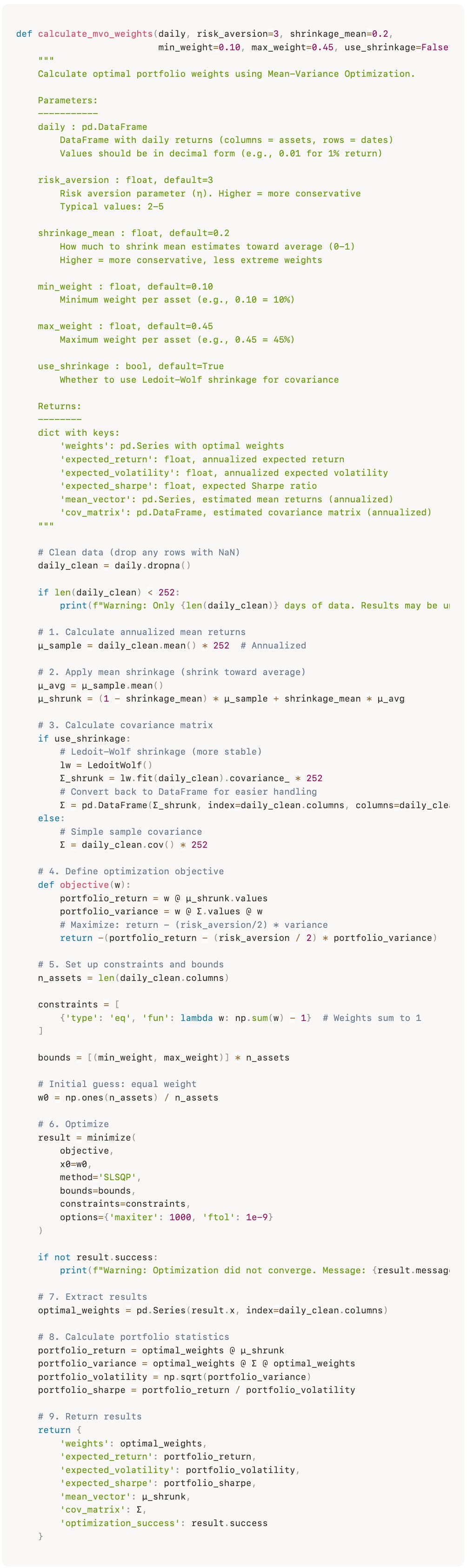
The implementation below uses scipy.optimize.minimize to solve this problem numerically. It also includes two optional refinements: Ledoit-Wolf shrinkage for the covariance matrix, and mean shrinkage that pulls return estimates toward their cross-sectional average. These regularization techniques can help when estimation error is a concern (though in our case, with only a handful of substrategies and years of daily data, they’re more of a safeguard than a necessity).
The code
The code is pretty straightforward:
Results
Now we can put the code above into a simple walk-forward loop: each year, we look back over the previous four years of daily returns, estimate the optimal weights, and then hold those weights fixed for the next year. We repeat this process as we roll forward through time.
Here’s what we get with minimum weight 0, maximum weight 60%:
Highlights:
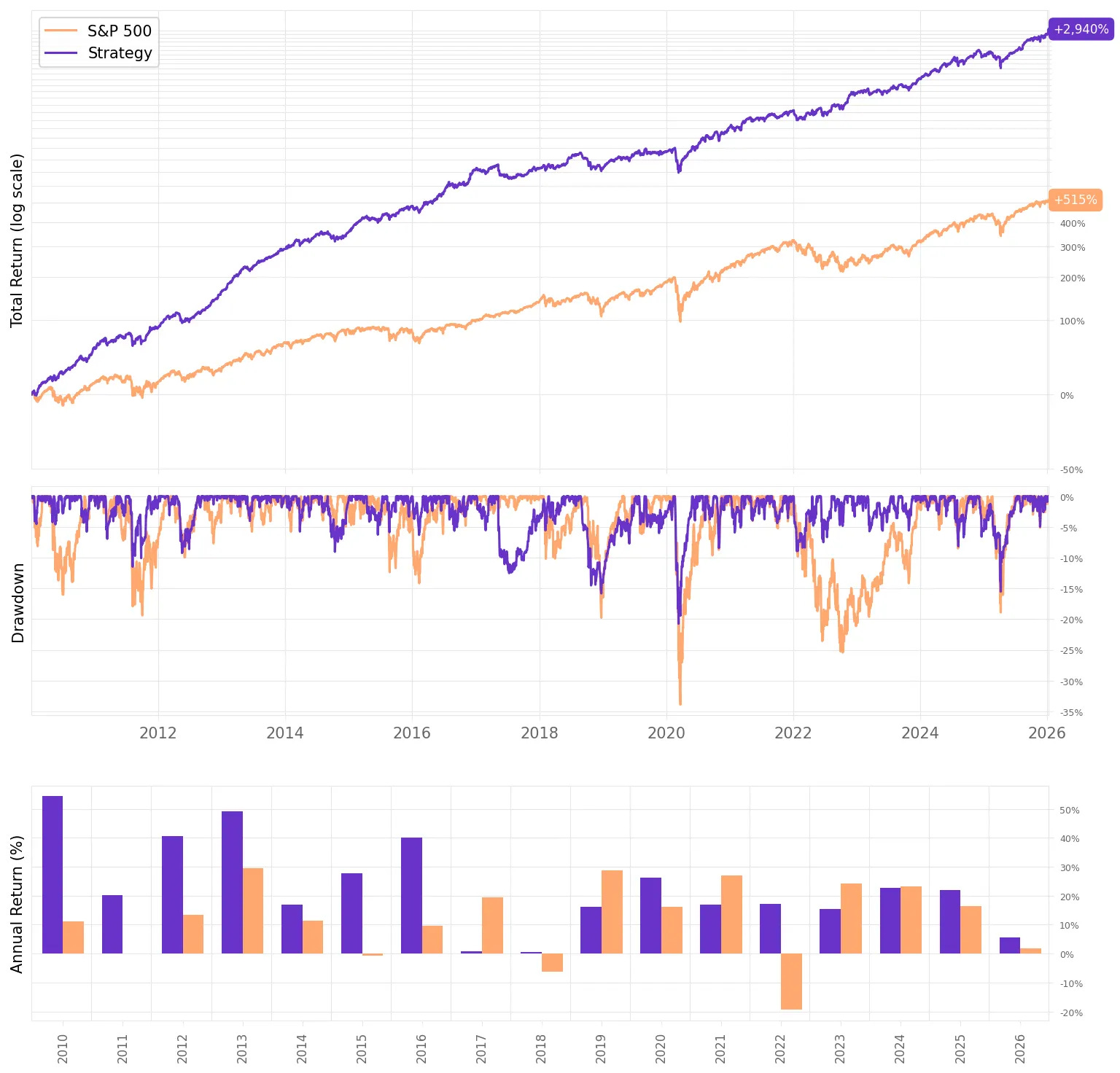
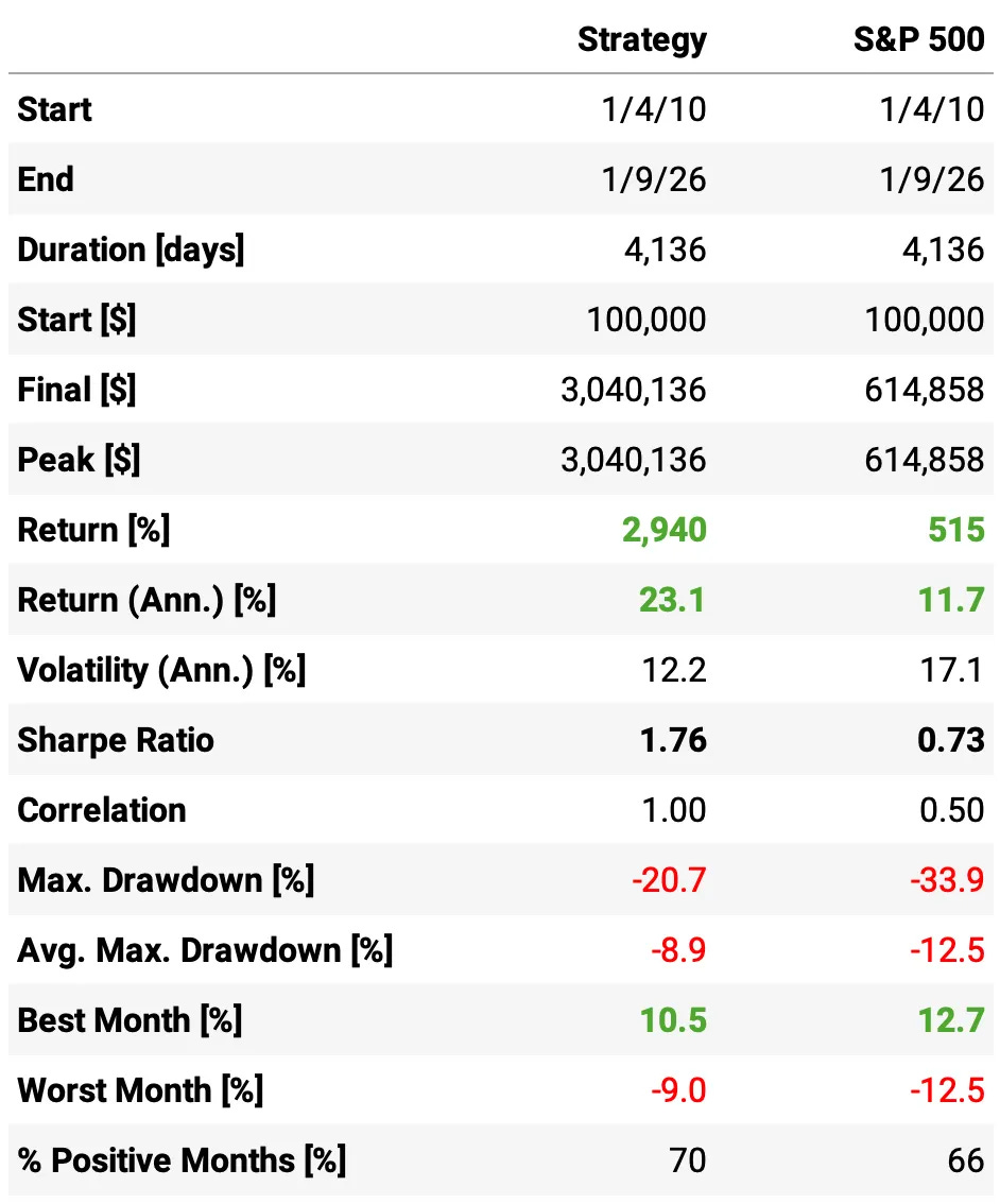
Higher return, same ballpark risk: MVO lifts annualized return to 23.1% vs 19.1% for equal-weights, while volatility stays low at 12.2% (vs 10.9%).
Sharpe improves even with slightly higher vol: 1.76 for MVO vs 1.66 for equal-weights, i.e., we’re getting more return per unit of risk despite taking a bit more volatility.
Much higher terminal wealth: $100k grows to $3.04M under MVO vs $1.75M under equal-weights (same 2010-2026 window).
Drawdowns don’t get worse: max drawdown is essentially unchanged/slightly better at -20.7% vs -21.4% for equal-weights, so the return boost didn’t come from accepting materially larger drawdowns.
Month-to-month consistency is the same: 70% positive months for both. The edge shows up mainly in the magnitude of gains, not a higher hit rate.
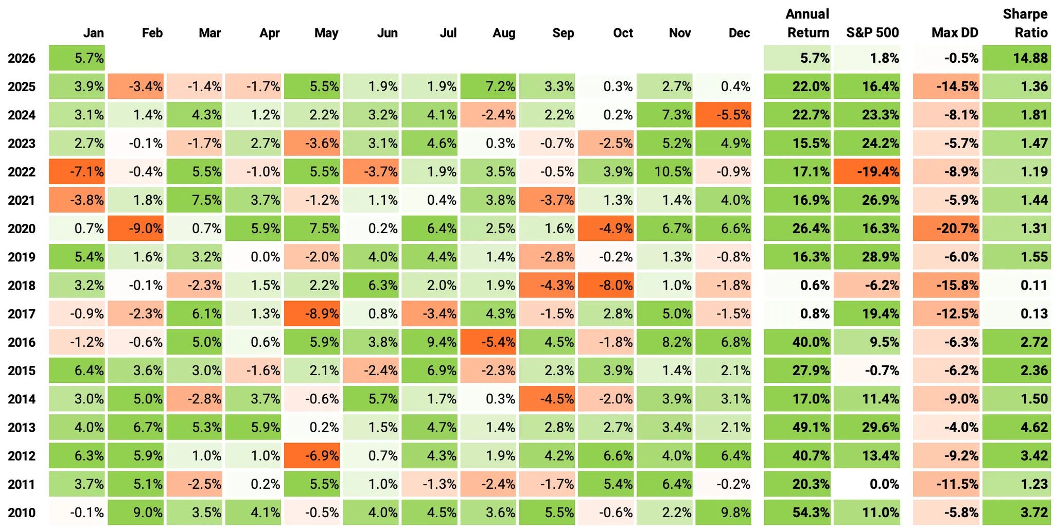
If we look at the monthly return distribution (2010-2026, 193 months):
70% of months were positive, with an average gain of +3.7%; 30% were negative, averaging -2.5%.
The best month was +10.5% and the worst month was -9.0%.
The “typical” month is strong: median = +2.0%; the middle 50% of outcomes sits between -0.5% (25th pct) and +4.3% (75th pct).
Volatility at the monthly level is moderate: std = 3.6%, with an overall mean = +1.85% per month.
Streaks: the longest positive streak was 21 months (Jun’12 → Feb’14); the longest negative streak was 3 months (Feb’25 → Apr’25).
The distribution is mildly asymmetric: skew = -0.40 (slightly more downside tail), with kurtosis = 0.22 (not especially fat-tailed).
Looking at the Fama-French 3-Factor risk model:
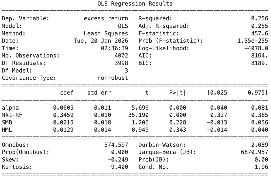
Alpha: 0.0605% per day → annualized ≈ 15%, highly significant (t = 5.70, p < 0.001): strong abnormal returns not explained by FF3 factors.
Market beta (Mkt–RF): 0.346, highly significant (t = 35.19, p < 0.001): meaningful, but not huge, exposure to the equity market (about one-third beta).
SMB (Size): 0.0215, insignificant (t = 1.21, p = 0.228): no reliable size tilt.
HML (Value): 0.0129, insignificant (t = 0.95, p = 0.343): no reliable value/growth tilt.
Explained variation: R² = 0.256: FF3 explains ~26% of daily return variation; the majority is still strategy-specific.
Final thoughts
We started with Markowitz’s 70-year-old insight — that diversification isn’t just intuition, it’s algebra — and applied it to a simple problem: allocating capital across three geographic variants of a mean-reversion strategy.
The results speak for themselves. Even the naive equal-weight portfolio delivered a +1.6 Sharpe by exploiting the remarkably low correlations across markets. But mean-variance optimization pushed it further: 23.1% annualized returns, a +1.76 Sharpe, without increasing drawdowns. The Fama-French regression confirmed what we hoped: a highly significant annualized alpha, minimal factor exposure, and only 26% of returns explained by standard risk factors. The rest is ours.
This is just the beginning. There’s plenty of room to explore:
More sleeves: add new geographies, signals, or timeframes to increase diversification degrees of freedom.
Smarter constraints: cap turnover, limit year-to-year weight changes, or impose risk budgets per sleeve to reduce allocation whiplash.
Risk overlays: simple beta hedging or volatility targeting can further stabilize the equity curve.
Markowitz was right: if we knew the future, we’d bet everything on one horse. We don’t, so we diversify, optimize, and let the math do the heavy lifting.
As always, I’d love to hear your thoughts. Feel free to reach out via Twitter or email if you have questions, ideas, or feedback.
Cheers!
We’re building a private community for systematic traders. A place to explore ideas, exchange insights, and tackle the real technical and strategic challenges of building robust trading systems… from signal research to execution and risk.
Enrollment reopens at the end of this month. Join the waitlist below to be the first to know when new seats open:
Love the emphasis on covariance being more critical than mean estimation for portfolio performance. The cross-geo correlation data (0.08 US-Canada, 0.10 Canada-Australia) is surprising low and creates real diversification value. That jump from 1.66 to 1.76 Sharpe with MVO shows proper allocation matters even when you're only dealing with a few sleeves instea of hundreds of individual names.
Hi, thanks for the interesting post. What does it mean that the equal weight is rebalnced annually?
If I understand it correctly, it means that the actual weights change throught the year while for the mean-variance portfolio the weights are constant for a year which mean that everyday you have to rebalance your portfolio daily in order to keep the weights constant. Thus, in the comparison between the 2 portfolios in reality there is a drag in the mean-variance one due to daily rebalance, correct?