The Bitter Lesson

Applying Deep Learning to Enhance Momentum Trading Strategies in Stocks

Richard Sutton, pioneer of reinforcement learning and a founding figure in modern AI.

The idea

“The biggest lesson that can be read from 70 years of AI research is that general methods that leverage computation are ultimately the most effective, and by a large margin.” Richard Sutton.

Richard Sutton is one of the greatest minds of our time. He is a founding figure in modern AI and a pioneer of reinforcement learning, the framework behind many of today’s most advanced intelligent systems. His work laid the foundations for agents that learn not from instruction, but from experience. A recipient of the Turing Award (the “Nobel Prize of Computing”), Sutton's influence is profound, reshaping how we think about learning, intelligence, and progress in AI.

In his landmark 2019 essay The Bitter Lesson, Sutton delivers a hard truth distilled from 70 years of AI research: methods that scale with computation, like search and learning, consistently outperform approaches that rely on built-in human knowledge. While it may be tempting to design systems that reflect how we think we think, history has shown that progress comes instead from embracing general-purpose algorithms and the exponential growth in computing power. It's a lesson many resist… until reality beats them over the head with it.

Human intuition may offer short-term gains, but brute-force computation ultimately wins.

This week, I’m going to write about this idea—and a failed experiment. But don’t be misled: the absence of a successful first result doesn’t mean the idea should be dismissed. On the contrary, this is the most important concept I’ve shared here so far. In fact, the core of The Bitter Lesson is one of the most important ideas in the history of computer science.

You’re probably already seeing where this line of reasoning leads. Many quantitative systems are built around rule sets that mimic human thinking. But Sutton’s core argument is that, in the long run, general-purpose algorithms that scale with compute will always outperform hand-crafted, human-informed approaches. He’s essentially saying that trying to manually craft trading rules is a waste of time. It might have worked in the past, but it won’t keep working much longer.

It’s a controversial point, I know. Let’s dive in.

As many of you have requested, I’ll be sharing some of my codebase in a course. It’s almost ready and should be finished in the next week or so. I’ve created the page below to explain the course content, who it’s for, and to answer the main questions about it. If you have any additional questions, feel free to send me an email.

Now, to the article!

Thoughts from an ex-Senior Quant from Citadel

Richard Sutton is also a personal hero. I devoured his Reinforcement Learning book—the definitive guide in the field—while taking the Reinforcement Learning and Decision Making class in grad school. In that class, under the guidance of the great professors Charles Isbell and Michael Littman, I developed the habit of reimplementing influential academic papers to deepen my understanding. It was my favorite course during my Master’s.

A few weeks ago, while watching the presentation "Deep Order Flow Imbalance: Extracting Alpha at Multiple Horizons from the Limit Order Book”, three minutes in, I started listening to Nicholas Westray make Sutton's Bitter Lesson point.

Westray, an ex-Senior Quant at Citadel (now at Point72, I think), explains Sutton's article and states the idea of his research: to forecast returns directly from raw limit order book (LOB) data, leveraging computation over domain knowledge.

His research shows that yes, using order flow data derived from raw limit order book data, a massive dataset, and a lot of compute power can indeed result in a model that can predict short-term returns.

It's a great talk worth listening to. Here are the paper and the slides for those who are more curious.

My first thought was to reimplement Westray’s paper as a learning exercise—something I picked up from Isbell and Littman in my Reinforcement Learning class. (Coincidence or not, one of the first papers I ever reimplemented was Sutton’s seminal work on temporal difference learning.)

I also wondered whether a simpler version of the idea might have profitable applications in less competitive corners of the market. There's only one way to find out: test it.

But as I read the paper more carefully, I realized this is a much larger project. Unfortunately, I don’t have the free time to tackle it in just a few weeks. It’ll take longer.

That led to my second thought: can we build a toy project instead? The idea is the same: throw a lot of data and compute at a return prediction problem to put Sutton’s Bitter Lesson to the test. Toy problems are also great learning tools.

Back in the day when OpenAI was still non-profit, I spent my fair share of time solving OpenAI Gym environments to learn deep reinforcement learning. I know the value of implementing toy projects.

Choosing a paper

If not Nicholas Westray's paper, which paper should I put to test? That was the next question. I have a library with over 100 papers I want to implement. It will take me many years, and I don't believe I will ever finish, because the library keeps growing.

Navigating through the library is hard, so I turned to Google and searched for “deep learning momentum stocks”. Why these terms? Simple: “deep learning” accounts for the lots of compute power & learning algorithms from Sutton's Bitter Lesson, and “momentum” is one of the most persistent anomalies in “stocks”. The top three results:

1. Slow Momentum with Fast Reversion: A Trading Strategy Using Deep Learning and Changepoint Detection, from Kieran Wood, Stephen Roberts, and Stefan Zohren

2. Dissecting Momentum: We Need to Go Deeper, from Dmitry Borisenko

3. Applying Deep Learning to Enhance Momentum Trading Strategies in Stocks, from Lawrence Takeuchi and Yu-Ying (Albert) Lee

Strategy performance from Slow Momentum with Fast Revision paper

Strategy performance from Dissecting Momentum paper

Strategy performance from Applying Deep Learning to Enhance Momentum paper

The first two papers look far more interesting, but are also longer-term projects to implement. On top of that, they involve too much feature engineering for my taste, especially Borisenko’s work, which somewhat defeats the purpose of using deep learning. Feature engineering depends heavily on human expertise, which contradicts the very lesson Sutton emphasized.

Now, the third paper has a different issue in my view: it seems too simple, almost too good to be true. The dataset is straightforward, the features are easy to derive… so where’s the catch? Still, simplicity means speed, so let’s start by testing this one.

The paper

Here are the key points for implementing the paper. For all details, check the original.

Data

Sample Selection

• Universe: U.S. stocks on NYSE, AMEX, NASDAQ.

• Exclude stocks priced below $5 to avoid microstructure noise.

• Training: 1965–1989 (848,000 samples), Testing: 1990–2009 (924,300 samples).

Input Variables and Preprocessing

• Input (33 features):

  • 12 monthly returns from months t−13 to t−2.

  • 20 daily returns from month t.

  • 1 January dummy variable.

• Convert returns into cumulative returns and z-scores for cross-sectional normalization.

• Target labels:

  • Class 1: returns below the monthly median.

  • Class 2: returns above the monthly median.

The model

Model and Training

• Use stacked RBMs to form an autoencoder, pretrained layer-wise.

• Compresses input to a low-dimensional feature space, then passes it to a feedforward neural network (FFNN) for classification.

• Final model is fine-tuned using backpropagation.

Architecture Specification

• Conducted grid search with hold-out validation (1965–1982 train / 1983–1989 validation).

• Final architecture: 33-40-4-50-2:

  • 33 inputs → compressed to 4 → classified into 2 classes.

• Justification: balance performance and complexity. No gain from deeper models.

Implementation

The full implementation is also available on GitBook for a better code browsing experience.

1. Data

In our replication, we will use daily stock prices from January 1, 1990, to today, obtained from Norgate data. Norgate provides a high-quality survivorship bias-free daily data for the US stock market that is very affordable. For more information on how to acquire a Norgate data subscription, please check Norgate website.

The first step is to retrieve the data for a given symbol:

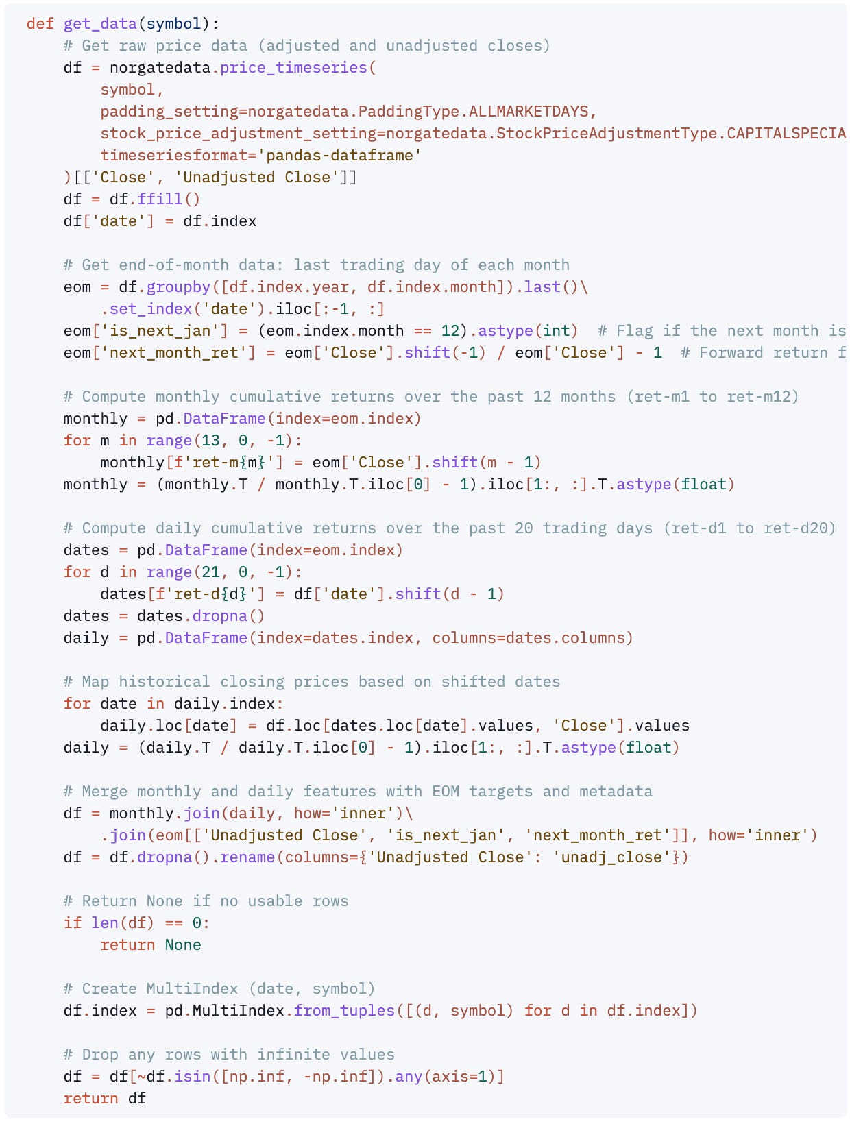
The function get_data(symbol) retrieves daily price data for a given stock symbol using Norgate, then constructs a feature-rich DataFrame indexed by (date, symbol) for use in predictive models. It calculates monthly cumulative returns (ret-m1 to ret-m12) based on end-of-month closes and daily cumulative returns (ret-d1 to ret-d20) over the last 20 trading days. It also includes the unadjusted close price, a binary flag is_next_jan indicating if the next month is January, and the forward return for the next month (next_month_ret). The function ensures no missing or infinite values and returns a clean, multi-indexed dataset ready for modeling.

We can check it with a call like get_data('AAPL'):

Data for AAPL

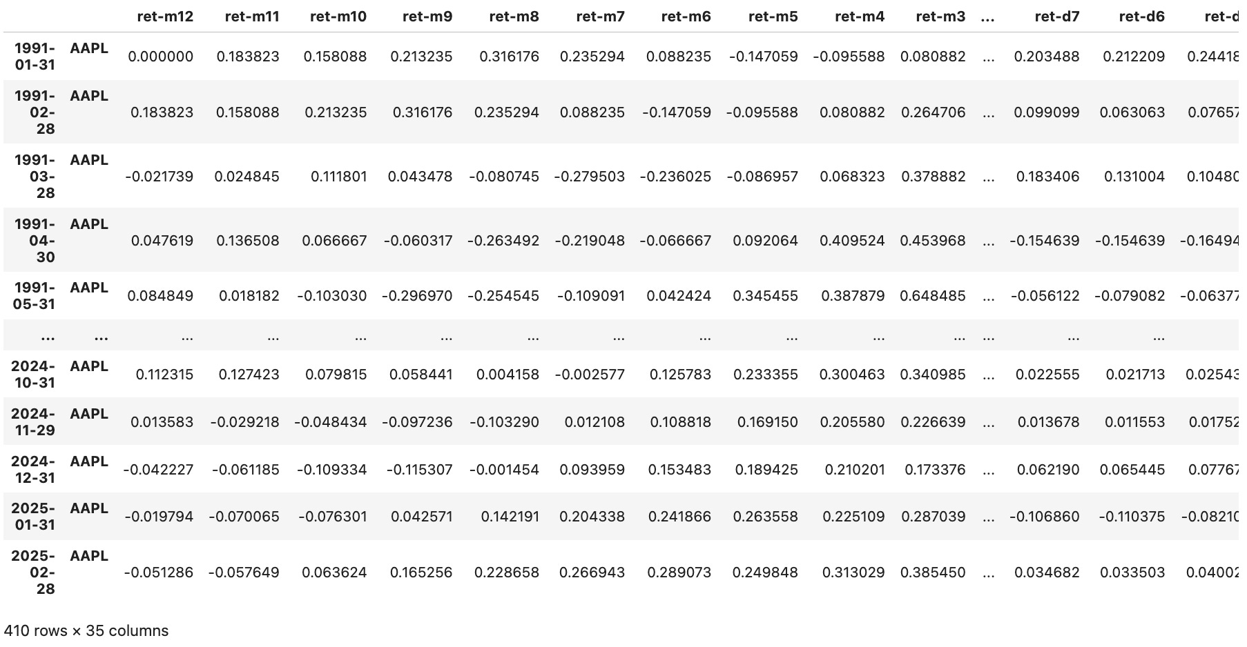
Now, retrieving all data is straightforward:

In about 30 minutes, we are ready to continue.

2. Pre-processing

Before training the model, we apply several pre-processing steps to clean the data, standardize features, and define the target variable:

We first filter out low-priced stocks (unadjusted close ≤ $5), which are often illiquid and noisy. Then, we apply cross-sectional z-score standardization to all features (excluding the last two columns) on each date to normalize them. The target variable is defined as a binary label: 1 if the next month’s return is above the median return for that date, and 0 otherwise. We also preserve the raw (unstandardized) version of the last feature (is_next_jan) and the original forward return for later analysis. All components are then combined into a single DataFrame for model input.

3. Cross-validation splits

To evaluate model performance over time, we implement a rolling-window cross-validation framework tailored for time series data:

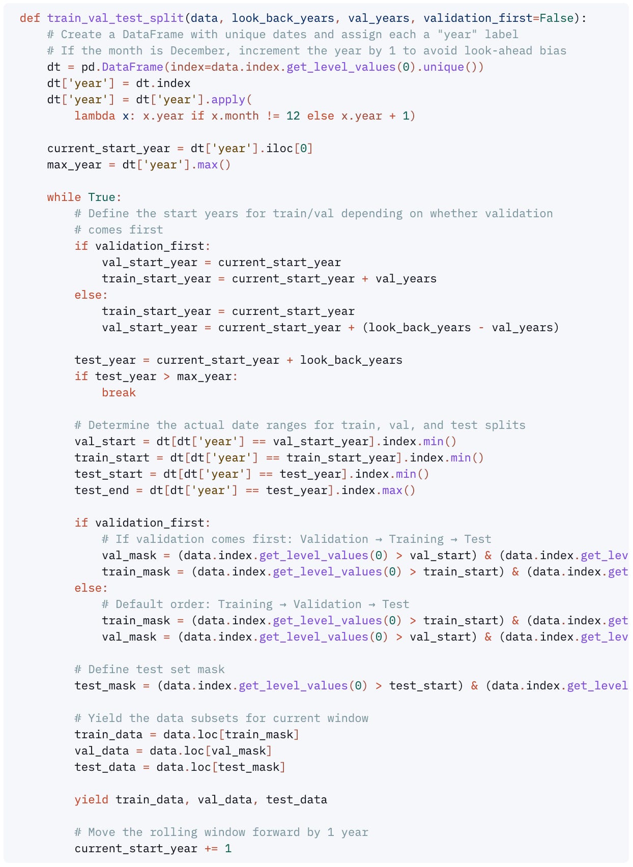
The train_val_test_split function generates chronological train/validation/test splits by sliding a multi-year window forward one year at a time. For each iteration, it defines a training period, a validation period, and a test year—ensuring no data leakage. We can choose whether to place the validation set before or after the training set using the validation_first flag. This approach mimics a realistic backtesting setup and provides out-of-sample evaluation across multiple time periods.

We can verify that the datasets are being generated correctly with the following code:

Train, validation, and test datasets

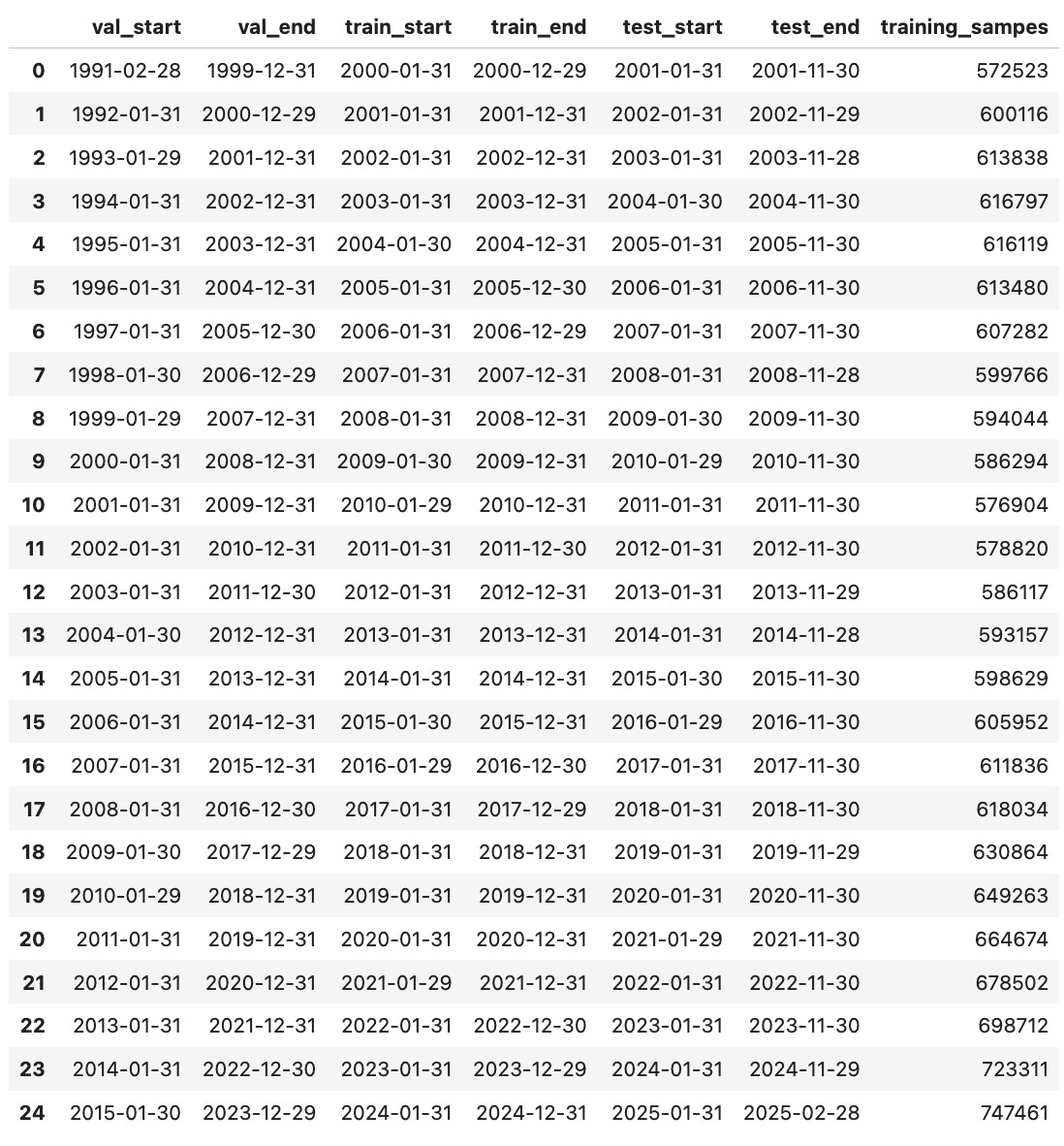
Now, we are ready to work on the model.

4. The model

We define a simple feedforward neural network (FFNN) architecture to classify the pre-processed features into two classes, as specified in the paper:

The FFNN model consists of three hidden layers with ReLU activations, followed by a final output layer that produces logits for binary classification. The input layer expects 33 features, which are transformed through progressively deeper representations: from 40 units, to 4, then to 50, before reaching the final output layer with 2 neurons. The model returns raw logits, which are suitable for use with CrossEntropyLoss, a standard loss function for multi-class classification tasks.

In the original 2013 paper, Takeuchi and Lee used a stacked autoencoder built from restricted Boltzmann machines (RBMs) for pretraining, which was common at the time. They pre-trained the encoder (33→40→4) to extract features and then attached a feedforward classifier (4→50→2) on top. Our model directly implements the final architecture they found optimal through cross-validation, bypassing the pretraining phase.

The reason we can now skip RBMs and pretraining is due to major advances in hardware (GPUs/TPUs), software (PyTorch, TensorFlow), initialization methods, and optimization algorithms (like Adam). These allow deep neural networks to be trained end-to-end from scratch efficiently, even on noisy financial datasets. In contrast, a decade ago, training deep nets from scratch often resulted in poor convergence, which is why unsupervised layer-wise pretraining with RBMs was widely used to help the network learn useful representations before supervised fine-tuning.

We can verify that our architecture works using the following code:

The code builds a PyTorch DataLoader from a DataFrame, converting features and labels to tensors for training. It retrieves one mini-batch, checks the shapes, and runs a forward pass through the FFNN to verify the model works as expected. We should see something like this:

Now, let's move to training.

5. Training

We now define the training loop used to optimize the model parameters using the training and validation sets:

The train function performs mini-batch training of the FFNN model using the Adam optimizer and cross-entropy loss. It tracks performance on both the training and validation sets, saving the model weights that yield the lowest validation loss. After training for a specified number of epochs, it returns the best-performing model along with key metrics such as validation loss, accuracy, and the epoch at which the best performance was achieved.

We now generate predictions and rank stocks by model confidence:

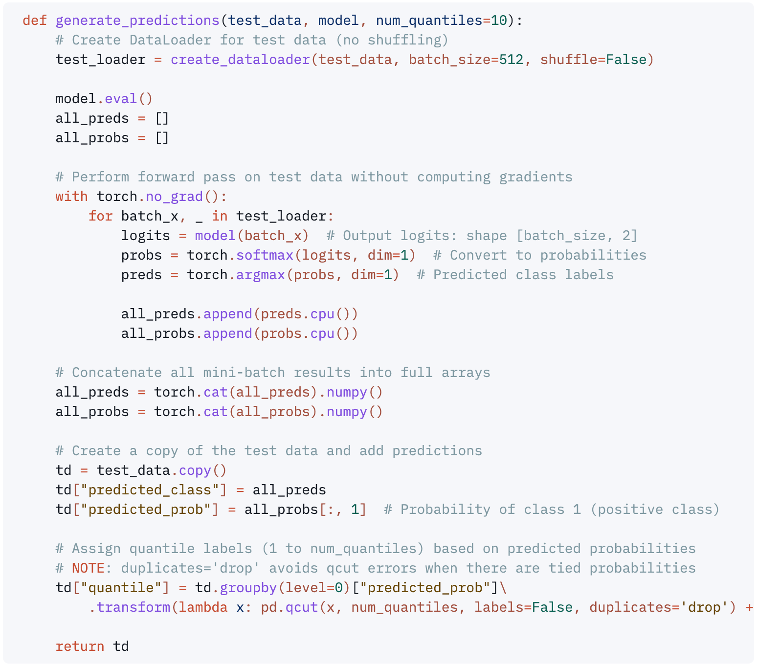
The method above generates model predictions on the test set by applying the trained network to each mini-batch and collecting the predicted classes and class probabilities. It appends these outputs to the original test DataFrame and assigns each example to a quantile bucket based on its predicted probability of belonging to class 1. This enables cross-sectional ranking of stocks by confidence level, which is useful for evaluating strategy performance by signal strength.

We now run rolling-window training and evaluation to collect predictions and track model performance over time:

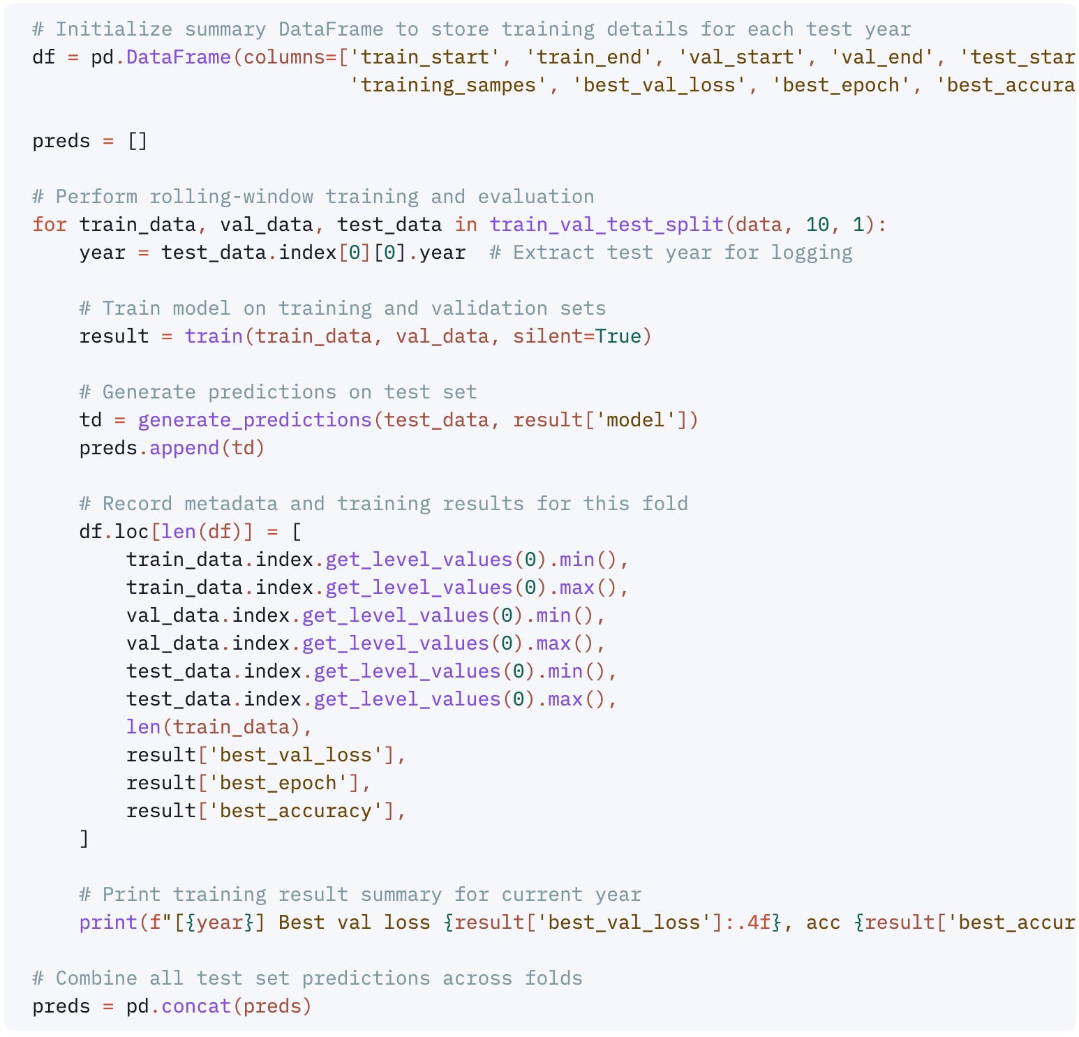
Running the code above will take a bit over an hour. We should see something like this:

The DataFrame that tracks the performance should record something like this:

Results from training the model

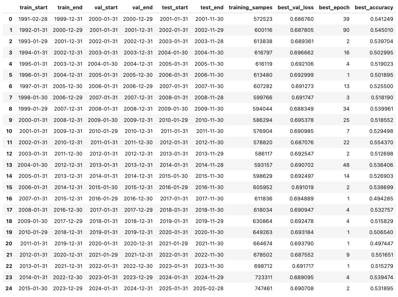
Now, we are ready to see the results.

Results

Let's start reviewing the model's classification performance by analyzing the confusion matrix:

This code compares the true labels and the model’s predicted classes across the entire test set to compute a confusion matrix, which is then column-normalized to show the distribution of predictions per class. This helps assess whether the model is biased toward one class and how well it distinguishes between them. The results are visualized using ConfusionMatrixDisplay, with values shown as proportions for easier interpretation.

We should see something like this:

Confusion matrix

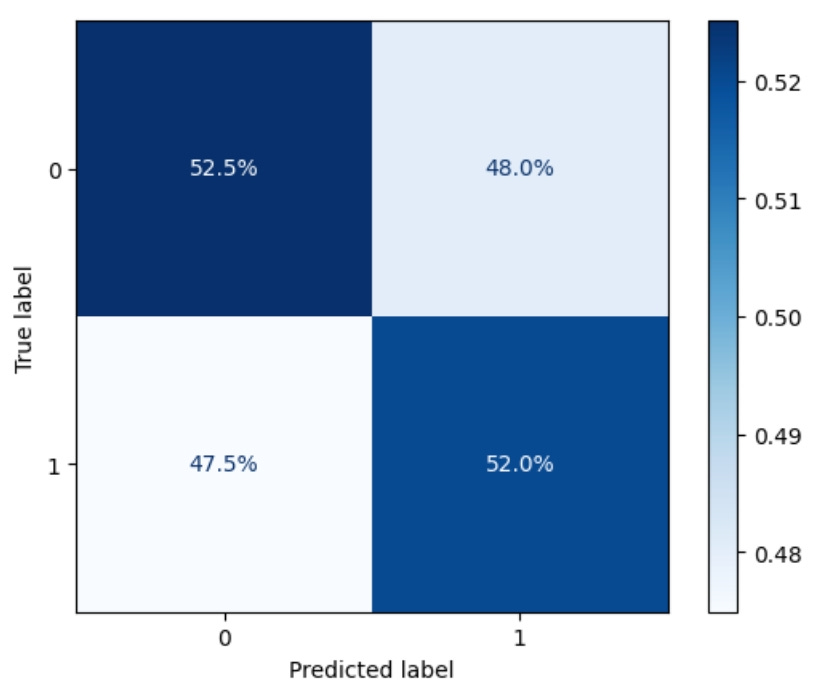
Highlights:

• The model is slightly better than random guessing, with ~52% accuracy for both predicted classes.

• It shows no strong bias toward one class—performance is symmetrical.

• This aligns with expectations for noisy financial datasets with low signal-to-noise ratios, where even a small edge (e.g., >50% accuracy) can be economically meaningful when scaled properly in a trading strategy.

We now compute the monthly long-short returns based on the spread between the top and bottom quantile predictions:

This snippet computes the average forward return for each quantile bucket on a monthly basis by grouping predictions by date and quantile. It then unstacks the results into a table where each column represents a quantile. Finally, it prints how many months are missing one or more quantiles, which can occur due to duplicates='drop' in qcut, highlighting potential data sparsity in certain months.

We now visualize the annualized average return by quantile to assess the relationship between predicted confidence and realized performance:

This code calculates the mean return for each quantile across all months, annualizes it, and plots it as a bar chart. The chart highlights how returns vary by model confidence:

Mean return for each quantile

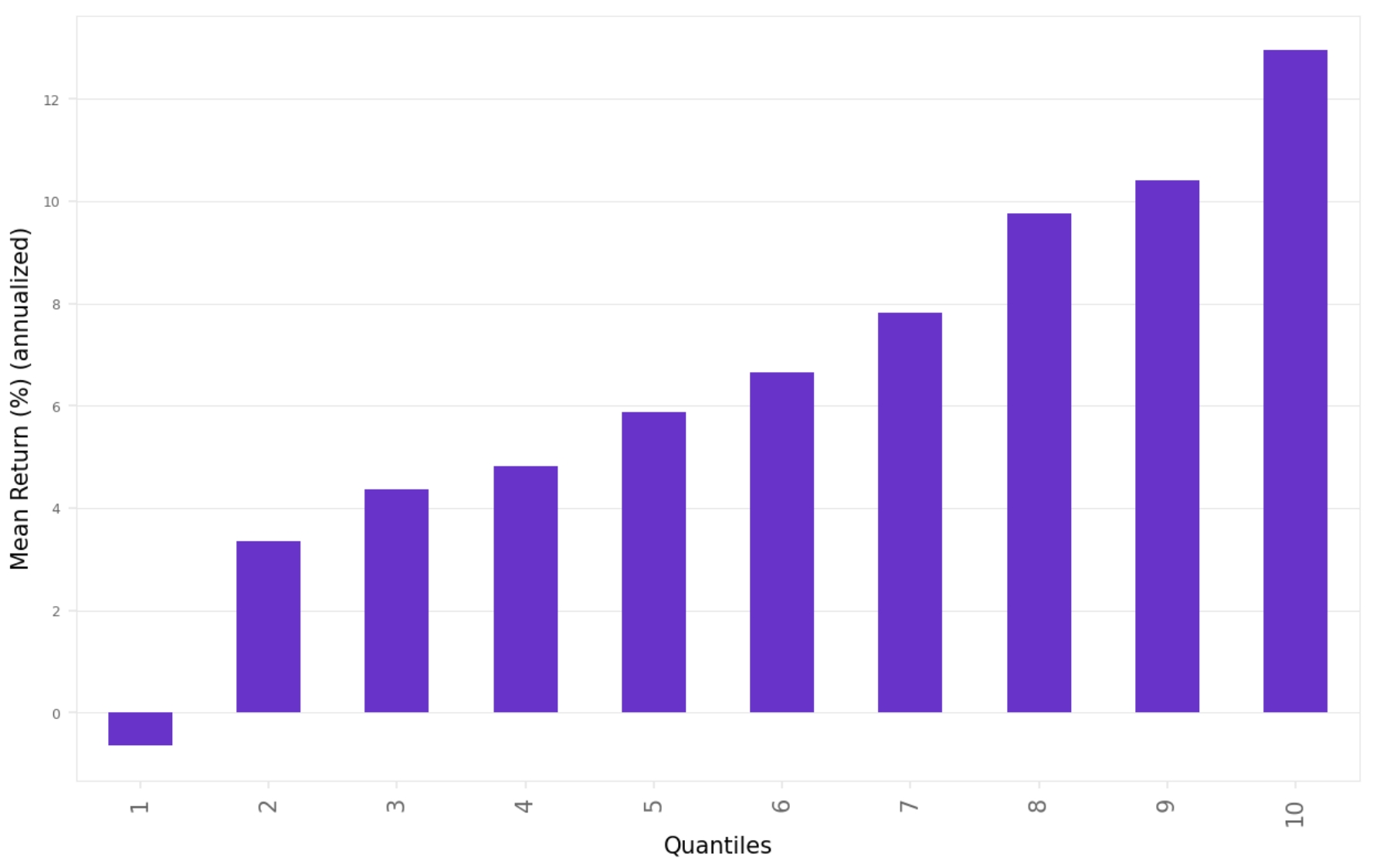
Highlights:

• Returns increase monotonically from quantile 1 to quantile 10.

• Quantile 1 has a negative return (-0.64%), indicating the model is correctly identifying poor-performing stocks.

• Quantile 10 shows the highest return at 13.0%, suggesting strong predictive power in selecting top-performing stocks.

• The spread between quantile 10 and quantile 1 is approximately 13.6 percentage points, which is economically meaningful.

• The results are not as good as described in the paper, but still, worth looking into it.

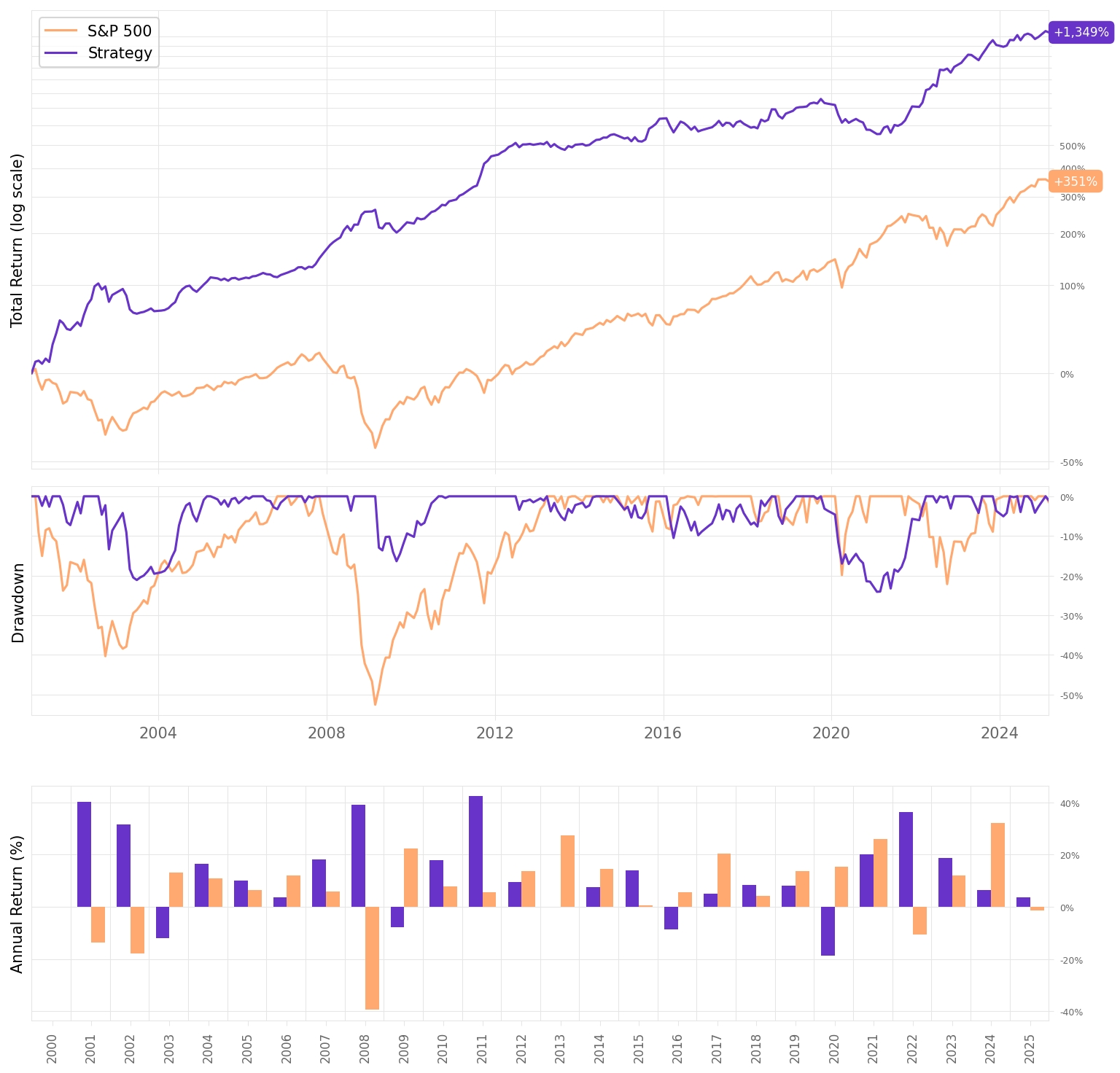
This pattern strongly supports the idea that the model’s confidence scores are informative, as shown by the authors in the paper. A long-short strategy (long top quantile, short bottom) would likely be profitable and consistent, as we can verify:

The snippet above generates the cumulative returns for the strategy. We can visualize it with one line, cumulative_rets.plot(logy=True), or if we add a bit more formatting and the benchmark:

Equity and drawdown curves

To get a summary of the backtest main stats, here's what we can do:

We should see something like this:

Summary of backtest stats

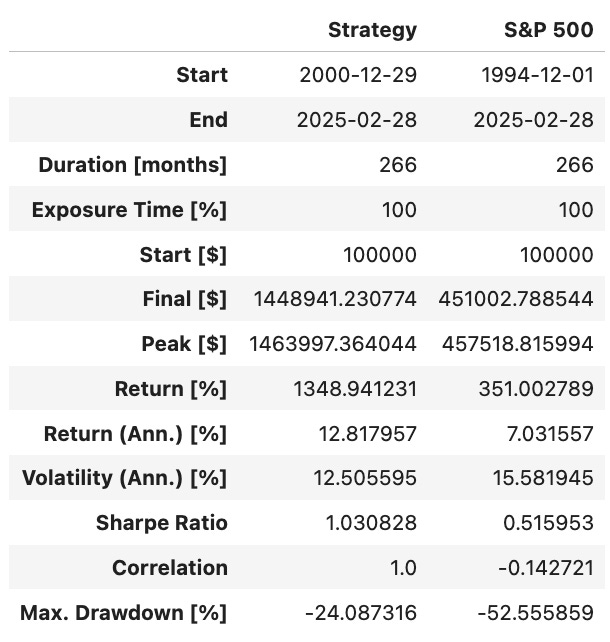
Overall, the strategy outperforms the benchmark across all key dimensions:

• Annualized return is 12.8%, nearly double the S&P 500’s 7.0%;

• Sharpe Ratio is 1.03, more than twice that of the benchmark, indicating superior risk-adjusted performance;

• Maximum drawdown is limited to 24%, less than half of the S&P 500’s 52.6%, reflecting strong downside protection;

• Correlation to the market is negative, offering valuable diversification benefits in a broader portfolio.

Final thoughts

While our implementation successfully demonstrated the viability of applying deep learning to momentum-based stock prediction, the results we obtained were a far cry from those reported by Takeuchi and Lee (2013). There are several likely reasons for this discrepancy. First, we used a different and significantly smaller dataset, both in terms of the number of stock-month observations and market breadth. Second, our time horizon was more recent and extended into a different market regime, potentially less favorable to momentum strategies. Third, unlike the authors’ original approach which involved unsupervised pretraining using stacked RBMs, we trained the feedforward network end-to-end using modern initialization and optimization techniques. Additionally, we adopted a rolling-window training and evaluation protocol, whereas the original study trained once on a large historical sample and tested on a fixed out-of-sample window. These methodological and structural differences, combined with evolving market dynamics, likely account for the performance gap.

Nevertheless, replicating the exact results reported by Takeuchi and Lee was never the true goal. The purpose of this project was to explore, in a simplified and more accessible setting, the core insight behind Richard Sutton’s Bitter Lesson: that general methods powered by computation outperform systems infused with human-crafted rules and domain expertise. Our toy example, despite its simplicity and the constraints we faced, served as a proof of concept for this idea. By throwing a clean pipeline, raw price data, and compute at the return prediction problem—without relying on hand-engineered financial indicators—we were able to extract signal and generate meaningful returns. In that sense, the experiment achieved what it set out to do: demonstrate that scaling learning systems and leaning into computation-first approaches can produce viable results even in challenging, noisy domains like financial markets.

I would love to tackle the other papers mentioned in this article right away. Unfortunately, I don't have time now. Their implementation will come later down the road.

Next, I believe we will tackle another interesting problem. Over the past months, I developed a system that is performing really well over the past month. Backtests looked great, so, we decided to deploy it in a small account.

It's being over 6 weeks and the system is killing it: it has deliverd over +3% vs. -9% the S&P 500. It has completed over 100 trades, so we have a minimally sufficient sample size to run some statistical tests and decide whether to continue collecting more data or scale it right away. What kind of analysis should we run to make a rational decision? That's what we will cover next.

As always, I’d love to hear your thoughts. Feel free to reach out via Twitter or email if you have questions, ideas, or feedback.

Cheers!