The Unintended Consequences of Rebalancing

How a simple rebalancing strategy boosts Sharpe from 1.0 to 1.30

The California Gold Rush

The idea

“I picked up one or two pieces and examined them attentively... I then collected four or five pieces and went to Mr. Scott... I said, ‘I believe this is gold.’” James W. Marshall.

He found gold… and died broke.

James W. Marshall unintentionally sparked one of the greatest migrations in American history. In 1848, while building a sawmill on the American River, he noticed a few glimmers in the water, triggering the California Gold Rush and forever altering the American West.

Back then, finding gold was easy. With little more than basic tools, everyday people could strike it rich. Some did (Marshall wasn’t one of them). But as more prospectors arrived, the easy gold disappeared. The shallow deposits anyone could reach with a pan were quickly depleted.

Still, despite the surge in miners and competition, gold production didn’t stop… it soared. Why? Technological advances, global exploration, and industrialization.

I find the analogy between gold mining and alpha research fascinating. Like gold, early alpha could be extracted using simple models. But as more participants entered the market, the obvious opportunities vanished. Today, finding alpha with a basic model in a crowded market is as unlikely as finding gold in the American River with a tin pan. If something glitters, it's probably pyrite… fool’s gold.

Yet alpha production has never been higher. Why? Again: technology, globalization, and industrial scale. The biggest quant firms and hedge funds have made more money in the past decade than ever before.

---

This week, we’ll implement the paper “The Unintended Consequences of Rebalancing” by Campbell Harvey, Michele Mazzoleni, and Alessandro Melone.

Front-Running Strategy Performance Over Time, as reported by the authors

The paper explores how institutional investors are forced to rebalance frequently, and how these predictable flows create arbitrage opportunities for those willing to front-run them. The strategy is surprisingly simple.

In fact, the model is so simple it made me picture someone striking gold today with nothing but a shovel. I know, I'm very skeptical. Possible? Maybe. Likely? Well, read on and decide for yourself.

Here’s the plan:

1. We’ll begin with a quick summary of the paper

2. Then, we’ll show the results from replicating their approach

3. Next, we’ll combine this strategy with a base portfolio of mean-reversion strategies to highlight diversification benefits

4. Finally, we’ll discuss next steps

If you know basic Python and Pandas, you can replicate this paper in a few hours. It’s a great warm-up if you're thinking about joining the second cohort of the course, which opens again in August. We've had lots of interest lately… more details soon.

---

We’re building a private community for systematic traders. A place to explore ideas, exchange insights, and tackle the real technical and strategic challenges of building robust trading systems… from signal research to execution and risk.

Enrollment reopens in August. Join the waitlist below to be the first to know when new seats open:

---

Paper Summary

“The Unintended Consequences of Rebalancing” explores how mechanical portfolio rebalancing by institutional investors, often done at predictable intervals, creates systematic, exploitable price distortions in equity and bond markets. The paper shows that these flows not only move prices but also impose hidden costs on long-term investors while offering short-term profit opportunities to arbitrageurs.

Core Idea

Institutional investors (like pension and mutual funds) regularly rebalance portfolios, selling stocks and buying bonds when equities outperform, and vice versa. This activity, often driven by either Calendar rules (e.g., monthly rebalancing) or Threshold triggers (e.g., when allocations drift by a set %), creates predictable and recurring trading patterns.

The authors construct two signals:

• Threshold Signal: Measures when equity/bond weights deviate from targets

• Calendar Signal: Captures end-of-month rebalancing pressures

Both signals significantly predict next-day cross-asset returns (S&P 500 vs. 10-year Treasuries). For example, a one standard deviation increase in these signals (indicating equities are overweight) predicts a ~17 bps decline in equities the next day.

Why Does This Happen?

Large funds must rebalance due to internal mandates, even when doing so imposes costs. These trades are:

• Mechanical, not information-driven

• Predictable, especially near month- and quarter-end

• Unavoidable, due to structural portfolio rules

This creates price pressure, which reverts within ~2 weeks, suggesting temporary inefficiencies.

The cost? Estimated at ~8 basis points per year—which adds up to $16 billion annually, or roughly $200 per U.S. household. This is more than the annual fee of passive investing.

How to Exploit It

The authors build a simple long-short strategy that front-runs rebalancers:

• If signals show equities are overweight → short S&P futures, long bonds

• If signals show equities are underweight → long S&P, short bonds

The strategy achieves a Sharpe ratio > 1 over 1997–2023. Returns are statistically significant and robust to controls for momentum, macro conditions, sentiment, and volatility.

This is one of the rare papers that documents a market-wide return anomaly caused not by alpha-seeking traders, but by the systematic behavior of the institutions themselves.

---

Replicating the paper

Both the Threshold Signal and the Calendar Signal are derived from the weights of a balanced equity/bond portfolio (60/40).

Over time, returns from the S&P 500 and 10-year U.S. Treasury note futures cause these weights to drift away from the target 60/40 allocation.

• In the Threshold Signal, the portfolio is rebalanced back to 60/40 whenever the drift exceeds a specified threshold (δ).

• In the Calendar Signal, the portfolio is rebalanced back to 60/40 on the last business day of each month, regardless of the drift.

Both signals are computed iteratively, tracking how portfolio weights evolve and trigger rebalancing over time:

\(w^T_{t+1}= \begin{cases} 60\% & \text{if } |w^T_t-60\%|\ge\delta \\ w^T_{t+1}(w^T_t; R^{SP}_{t+1}; R^{10Y}_{t+1}) & \text{otherwise} \end{cases} \)

\(w^C_{t+1}= \begin{cases} 60\% & \text{if } t \text{ is the last day of the month} \\ w^C_{t+1}(w^C_t; R^{SP}_{t+1}; R^{10Y}_{t+1}) & \text{otherwise} \end{cases} \)

Here, w^C_t denotes the weights for the Calendar Signal, while w^T_t denotes the weights for the Threshold Signal. The formula that updates the weights as a function of previous weights and returns is:

\(w^j_{t+1}(w^j_t; R^{SP}_{t+1}; R^{10Y}_{t+1})= \frac{w^j_t(1 + R^{SP}_{t+1})} {w^j_t(1 + R^{SP}_{t+1}) + (1 - w^j_t)(1 + R^{10Y}_{t+1})}\)

Coding these signals is fairly straightforward. Two questions remain:

• What threshold values (δ) should we use for the Threshold Signal?

• How many days before month-end does the Calendar effect typically materialize?

Both questions are addressed through predictive regressions using different values of δ (for the Threshold Signal) and N (the number of days before month-end for the Calendar Signal):

Signal Calibrations

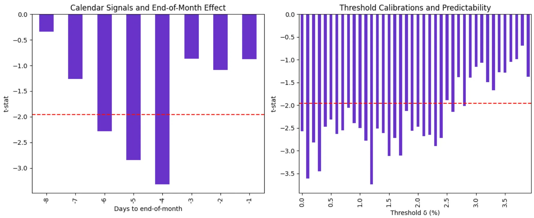
The calibration results guide two key modeling choices. For the Calendar Signal, we observe that the predictive power (t-stat) becomes statistically significant about 5 days before month-end, justifying the use of N = 5. For the Threshold Signal, predictability weakens beyond δ = 2.5%, so we average signals across all δ values from 0% to 2.5% in 0.1% increments to capture a representative rebalancer behavior without overfitting to a single threshold.

The strategy

The trading strategy takes a position in a S&P 500 futures contract and an opposite position in a 10-year Treasury note futures contract as follows:

\(R^{\text{Strategy}}_t=(R^{SP}_t-R^{10T}_t) \cdot w^{\text{Strategy}}_t\)

where the portfolio weight $w^{\text{Strategy}}_t$ is defined as the average of modified versions of the Threshold and Calendar signals. The modifications primarily involve rescaling, inverting the signal, and averaging, among other adjustments. See the paper for full details.

Running that leads to an equity curve pretty similar to what was reported:

Front-Running Strategy Performance Over Time (benchmark is rescaled to the same volatility, as done by the authors)

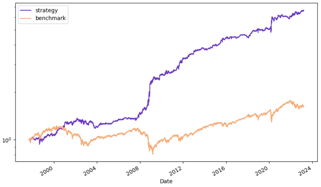
The Sharpe ratio we obtained was 0.94, which is close enough to the value reported in the paper. Tweaking the rescaling parameters and other small details might improve the results slightly. But that's not what we want to do next.

---

Adding the strategy to a portfolio

Now let’s assess the benefits of adding this strategy to a broader portfolio.

We'll use as a baseline the mean reversion strategy portfolio we've been trading (based on ideas we've shared here) for nearly a year.

Below are the baseline results before adding the new strategy:

Equity and drawdown curves of the portfolio of MR strategies (baseline)

Summary of portfolio statistics (baseline)

Monthly and annual returns (baseline)

As we've mentioned in previous articles, this is a strong portfolio, delivering more than twice the risk-adjusted returns of the S&P 500.

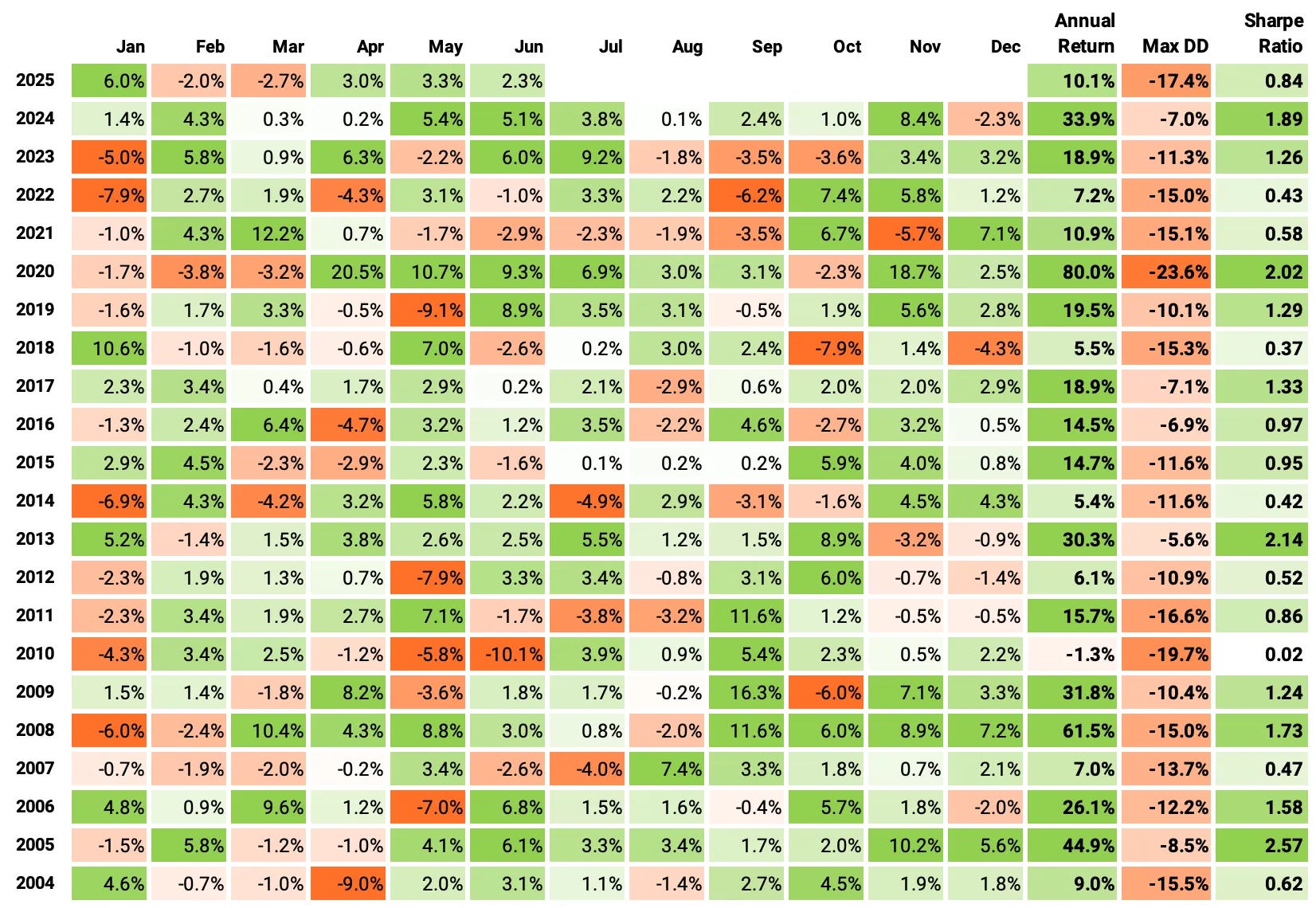
Now, let’s see how performance improves when we blend it 50/50 with the Front-Running strategy we just replicated:

Equity and drawdown curves of the portfolio of MR strategies (hedged portfolio)

Summary of portfolio statistics (hedged portfolio)

Monthly and annual returns (hedged portfolio)

Here are some key highlights:

• By adding the strategy to our portfolio, we increased the Sharpe ratio from 1.08 to 1.30

• Annual volatility dropped from 19% to 14%

• Maximum drawdown improved from 24% to 15%

• The average annual maximum drawdown fell from 13% to 8%

• The percentage of positive months rose from 66% to 71%

We gave up 2.5% in annual returns (from 20.6% to 18.1%) in exchange for significantly better downside protection and lower volatility.

Seems like a good trade-off. ;)

---

Final Thoughts

What started as a simple idea, front-running mechanical rebalancing flows, turned out to be surprisingly effective. The strategy alone delivers solid performance. But when paired with our mean reversion portfolio, it adds something even more valuable: resilience. Sharpe goes up, volatility drops, and drawdowns become shallower and shorter.

This is exactly the kind of research we like: economically intuitive, data-driven, simple to implement, and additive in a portfolio.

There’s still more to mine here. This idea could be extended across asset classes, refined with smarter execution, or combined with other signals. But even in its basic form, it looks like a real nugget of gold.

We’ll keep digging, both in future posts and in more depth inside the private community when Cohort 2 opens this August.

As always, I’d love to hear your thoughts. Questions, comments, feedback—just reach out via Twitter or email.

Cheers!

---

The first cohort of the course was a great success. Thank you to everyone who joined!Enrollment is now closed. The next cohort opens in August, with 50 more seats.Course participants also get exclusive access to our Community and Study Group.Join the waitlist below to be notified when enrollment reopens:

(I know, I need to update this landing page… as soon as I find time I will add more details about the course, the community, reviews from the 50 first users, etc :))

---

---