Triangulated Statistical Arbitrage

A 2.4 Sharpe signal built on asset networks

Pietro della Vecchia - The Philosophers (Ptolemy and Euclid with Their Pupils)

The idea

“Ratios which are the same with the same ratio are also the same with one another.” Euclid.

How can we say if something is cheap or expensive? Let’s borrow some ideas from an ancient book, written around 300 BC, to try to answer this question (and develop a trading strategy in the process).

The book in question is Euclid’s Elements, also known as the bible of geometry. It’s always amazed me how this little book, filled with common notions and propositions, is still so influential to this day.

A ratio isn’t a thing. It’s a relationship between two things. Euclid’s first axiom says that things equal to the same thing are equal to each other. V.11 (the intro quote) says the same is true of relationships.

But how can these self-evident truths help us reason about the value of things?

This week, we will develop a relative-value strategy called “Triangulated Statistical Arbitrage”. I first read about the overall idea in a series of six posts from Kris Longmore about statistical arbitrage (here’s the link to the series; Kris also has a Substack, which I recommend subscribing to!).

Kris did a great job describing the concepts, but he intentionally omitted the implementation details for obvious reasons. I took the broad methodology as I understood it and filled in the blanks.

Indicative implementation from Kris's article

My indicative implementation (comparable to Triangulated, consistency/depth aware, earnings unaware)

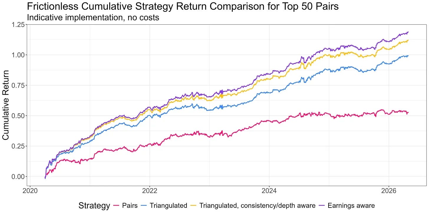
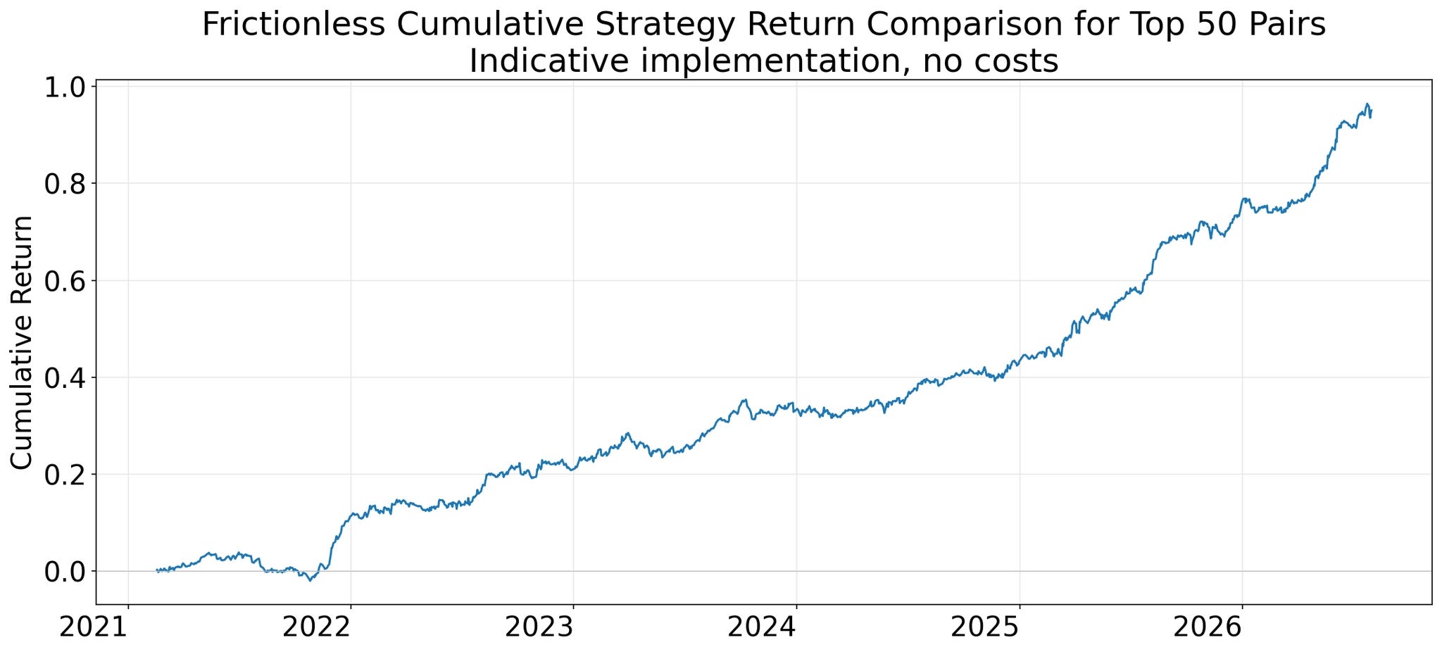
Although I am following the same overall approach as Kris, I arrive at different results: I am filling lots of blanks in the method he didn’t disclose.

In his articles, Kris said he has been trading this idea for the past few months; I will start trading it too, maybe write a follow-up piece with the live results. Let’s see.

Here’s our plan:

1. First, we will summarize what the strategy is: its main concepts

2. Next, we will review, step by step, how I specifically implemented the idea & the results I obtained

3. Then, we will review how I decided to build the asset network (the crux of the strategy)

4. Finally, we will wrap up with final thoughts as usual

Let’s get started.

---

---

The main concepts

1. The bet is convergence

Why “statistical” in statistical arbitrage? At first glance, some people might get confused about this: the term “statistical” is NOT because you use statistics to find price relationships that comove. It’s because convergence is not guaranteed.

There are so many articles and papers focusing on statistical tools (cointegration tests, optimal hedge ratios, Ornstein-Uhlenbeck processes, etc) rather than on the most important thing (pairs/basket selection), that the confusion is understandable. But we will show all these fancy tools are dispensable.

What actually drives prices to diverge and converge within certain pairs/baskets?

• Divergence comes from forced flows / price-insensitive participants: index rebalancing, hedging needs, liquidity requirements, some “situational unaware” fund manager was forced to sell, etc. They are not expressing a view. Thus, they create temporary mispricings.

• Convergence follows because if the two assets (or all the assets in the basket) share risk factors, that displacement is noise, not fundamentals. And noise mean-reverts once the market takes notice.

2. Measure the behavior you want, not a statistical property

If we are going to trade the spread of a pair of assets’ prices, the most important question we should answer is: does this spread diverge and converge in a tradable way? This is what we care about, not if the cointegration coefficient is X or Y.

The skeleton pipeline:

1. Start with pairs that make structural sense (for example, names from the same industry like two oil stocks, two banks, or two retailers): this is the most important step

2. Filter pairs that have stayed close together historically (persistence is important)

3. Filter pairs that have shown strong mean reversion (frictionless mean-reversion return)

4. Rank by some combination of those metrics

5. Take the top N to trade

(Don’t worry, I will be more precise about how I implemented these steps in the next section.)

Pairing statistically related but economically unrelated stocks is a very bad idea. Spurious relationships break down. If you bet on the convergence of pairs with no fundamental connection, it’s pretty safe to say that they will diverge permanently sooner or later, and you will end up at a loss.

Photo of the most famous cat in statistics

3. Three ways the pair form wastes a good signal

Trading pairs works, but it’s inefficient:

• You can only trade a fraction of the universe, especially if you have limited capital;

• The capital you do deploy is used inefficiently, because in a pair, usually only one leg is mispriced;

• You cannot aggregate the signal. 100 pairs do not involve 200 unique stocks (there’s a heavy overlap).

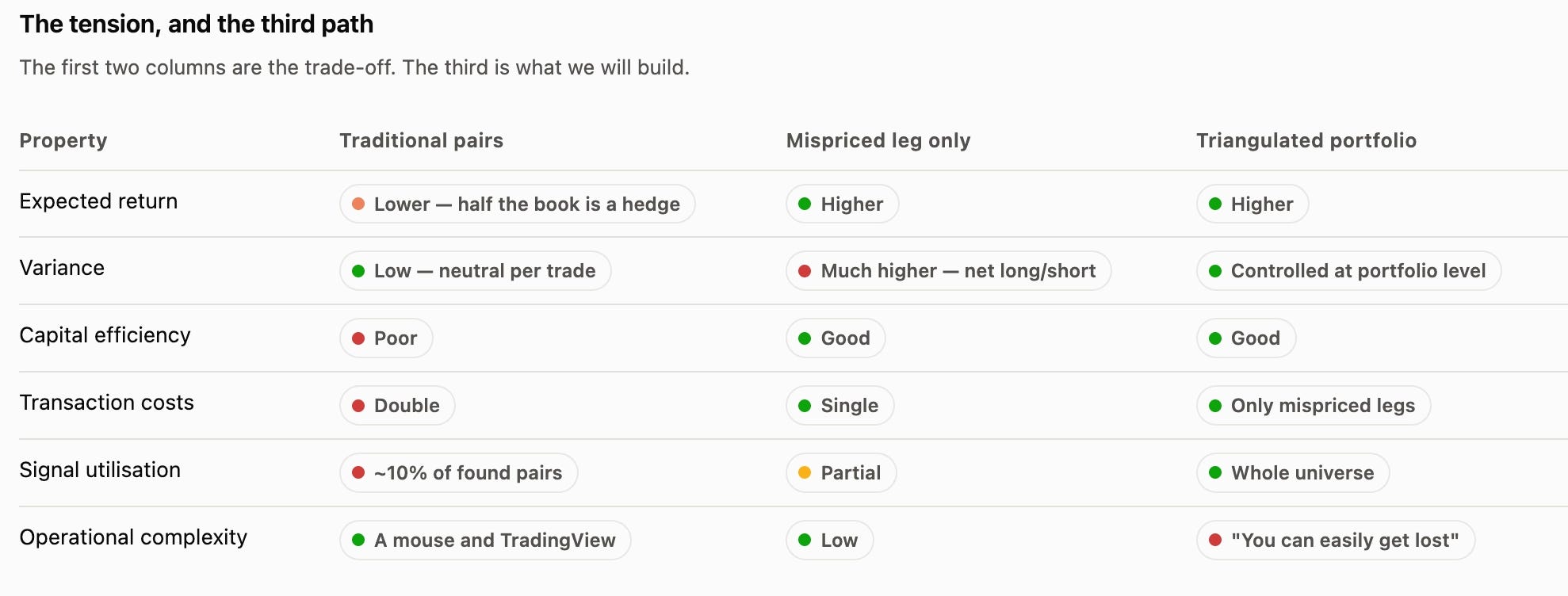
If trading pairs is inefficient, why not trade the mispriced legs only? Well, we would lose the dollar-neutrality, and the portfolio variance would grow significantly.

The solution is the triangulated portfolio: flattening pair signals into signals on individual assets, aggregating across many pairs, and constructing a portfolio whose market exposures cancel at the portfolio level rather than trade by trade.

Let’s see next what that means in detail.

4. Spreads as evidence, not trades

Let’s look into a basket containing six semiconductor stocks, all similar* to ASML:

* We will see how to get these similar stocks in the next section

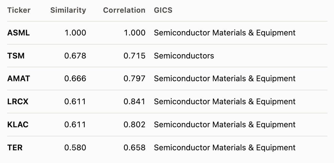
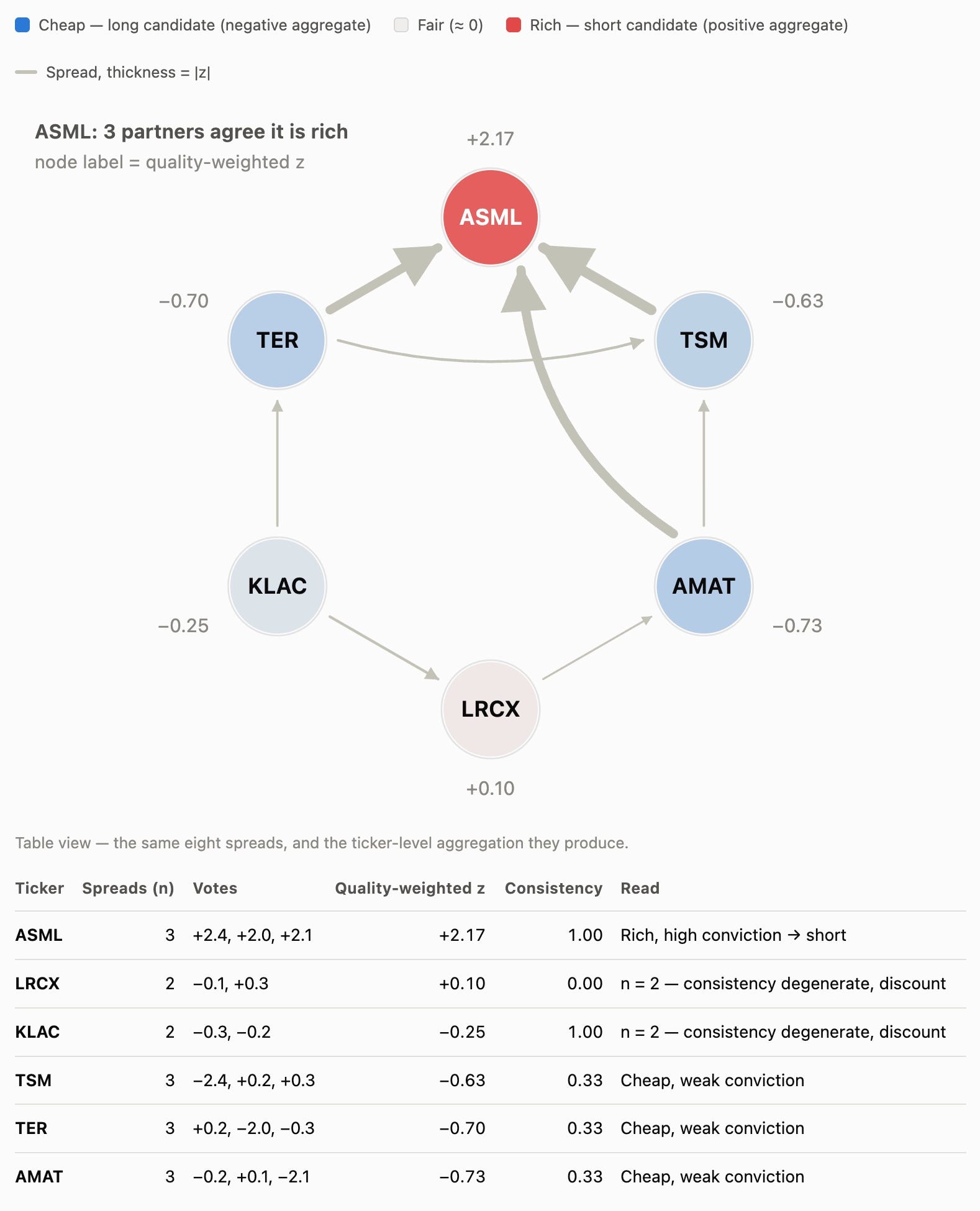
Now, let’s see this basket at a certain point in time. It’s kind of a network, where every spread connects the pairs in the network.

Imagine, now, that three spreads involving ASML are stretched (expensive), while every other spread not involving ASML is near zero. TSM, AMAT, LRCX, KLAC, and TER trade fairly against each other.

The network of overlapping spreads says something no single spread can: in our example, ASML is the mispriced stock:

Flattening

Now, we collapse each spread-level signal into two ticker-level votes of equal magnitude and opposite sign. One spread becomes two votes… we do it for every spread, then aggregate per ticker.

The votes in our semiconductor basket example

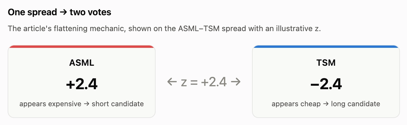
In our example, ASML appears in three spreads that all say rich: that’s a strong positive aggregate. TSM appears in three too, but only one says cheap. The others say roughly fair: the votes disagree! This is a weaker conviction, so probably not the mispriced leg.

Consistency

Taking consistency into consideration is important. We convert a ticker’s votes to +1 or -1, average them, and take the absolute value. Super simple:

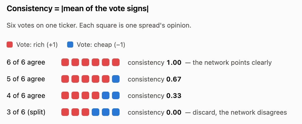
A ticker with a strong average signal but low consistency is probably not the mispriced leg. A ticker with a moderate signal but high consistency is the cleaner trade.

From signals to a portfolio

Strong negatives go into the long book, while strong positives go into the short book. We are no longer holding “one mispriced leg + one fair-valued leg” repeated many times: we are holding a portfolio of mispriced tickers only. Longs are cheap, shorts are rich, and both sides work for us.

• The effect concentrates in the extremes

• By sizing to net market exposure ≈ 0, we get the pairs-like portfolio variance reduction through portfolio construction rather than pair-by-pair hedging

• The aggregated pairs signal can go into a broader multi-factor long/short portfolio as just another factor

More

In the original six-part series, Kris goes deeper: he talks about incorporating the earnings calendar to avoid true repricings, incorporating news flow, seeing the network as a linear system, and more. Again, I recommend everyone check his great articles. The link to the first one in the series is here.

But with what I already shared (my understanding of his overall approach), I was able to get to a signal with 2.4 gross Sharpe (1.2-1.9 after cost, depending on the cost assumptions), so that’s a good place to stop and shift gears: now, let’s fill in the blanks and see some implementation details.

---

Filling in the blanks, step by step

“Pair selection is where the whole thing either lives or dies.” Kris Longmore.

In his articles, Kris mentions that starting with pairs derived from similar industries or sectors leads to a good baseline.

I tried GICS industry classification as a good place to start, but I couldn’t get a signal with a Sharpe ratio above 1.6.

Then, I tried a few innovative approaches to generate economically meaningful pairs, and that worked really well: the signal Sharpe reached 2.4. Here’s what I did that worked: