Volume Shocks and Overnight Returns
Can a +1.5 Sharpe strategy survive real-world frictions?
The idea
"Everything should be made as simple as possible, but no simpler." Albert Einstein.
Albert Einstein had a way of capturing deep truths in simple words. His quote is a reminder, especially relevant to us when building models. Stripping away unnecessary complexity is vital, but going too far risks oversimplification: a model that looks neat but fails to capture reality.
This week, we will implement the idea from the paper Volume Shocks and Overnight Returns, by Álvaro Cartea, Mihai Cucuringu, Qi Jin, and Mungo Ivor Wilson (2025, all from Oxford).
(By the way, sorry for taking so long to publish this piece… I’m in Bali for a 3-week blockchain conference for hardcore protocol engineers. I thought it’d be a good way to finally start dipping into crypto properly… It’s been a steep but rewarding learning curve… More on that soon!)
In practice, we’ll adapt the paper’s core insight rather than copy it wholesale. On one hand, we’ll simplify a key element of their setup that we believe can be expressed more cleanly without losing its essence. On the other, we’ll add back an important piece they left out — trading frictions and costs — because ignoring these can turn an elegant academic signal into an unrealistic strategy. The goal is to strike the right balance: simple enough to be practical, but rich enough to hold up in the real world. Or, as Einstein might put it if he were a quant: make it simple, just not “fantasy-backtest simple.”
Here's the plan:
First, we will quickly summarize the paper
Then, we will run the naive, simplified implementation
Next, we will model friction & trading costs and compare
Finally, after breaking the strategy, we will make it work again
As usual, we will wrap up with final thoughts and next steps
Course and Community: enrollments Open
As many of you requested, the 2nd cohort of the course is now live and open for enrollment.
It walks through my codebase step by step and is designed for readers who want to develop quant strategies using the same approach I’ve shared here.
You’ll find all the details—content, structure, pricing, and FAQs—at the link below. If you have any questions, feel free to reach out.
Enrollment also includes access to the private community and an ever-growing library of study groups. The code and full recording of the latest session (“Execution details of Intraday Momentum for ES & NQ”) are already available.
Paper summary
Core Idea
The paper shows that unexpected spikes in trading volume (“volume shocks”) during the day predict positive returns overnight — but not during the next trading session.
Stocks with large volume shocks earn significantly higher close-to-open returns.
This relationship is robust across firm sizes and persists after controlling for standard risk factors (market, size, momentum, reversal).
Importantly, intraday returns (open-to-close) show no such effect, highlighting a unique overnight premium linked to volume shocks.
Why Does This Happen?
The usual explanation — that high volume reflects investor attention, lowers cost of capital, and should boost returns — doesn’t fit. If it did, the effect would show up during the next trading day, not just overnight.
Instead, the authors argue:
Market frictions and constraints (liquidity, noise trading, institutional execution) delay full incorporation of information until the next morning.
Information flow after hours (e.g., earnings, news releases, sentiment shifts) interacts with the signal from volume shocks, amplifying the overnight effect.
Overnight risk premia: investors may demand compensation for holding positions across the less liquid, higher-risk non-trading period.
How to Exploit It
The trading challenge is that true volume shocks are only known after the close auction. The authors tackle this by predicting volume shocks during the day using linear and machine learning models (LightGBM, TabNet, etc.):
Predicted volume shocks can be used to build long-only overnight portfolios.
Even simple models capture ~90% of the “oracle” (perfect foresight) strategy’s Sharpe ratio.
Best ML models (TabNet) achieve ~97% of the oracle’s performance, with Sharpe ratios around 1.1 and annualized returns near 18%.
Crucially, trading only the high-volume side avoids liquidity traps, since low-volume stocks are harder to execute.
Naive simplified version
Instead of building complex ML models to forecast volume shocks, we’ll start with a stripped-down version that’s simple and actionable. The setup:
Signal timing: use trading volume information up to 3:45 pm, so trades can be placed with MOC orders (data from Polygon.io)
Portfolio construction: begin with a naive equal-weight implementation
Universe: run the strategy across the Russell 3000 stocks (data from Norgate)
Positioning: keep it long-only, consistent with the paper
Sorting: classify volume shocks into 10 quantiles (instead of 5) and trade only the top decile
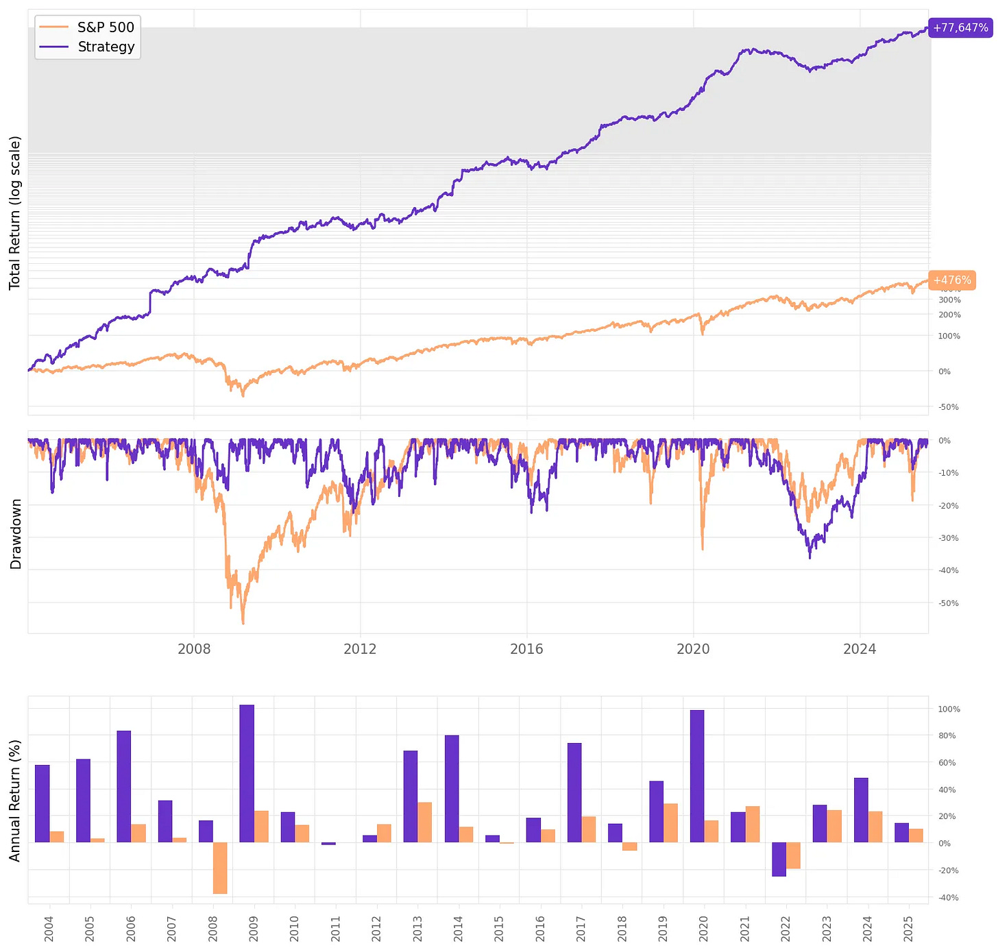
We will start with zero cost or friction. This is obviously unrealistic. But that's just to see what an unrealistic test looks like. Let's check the results:
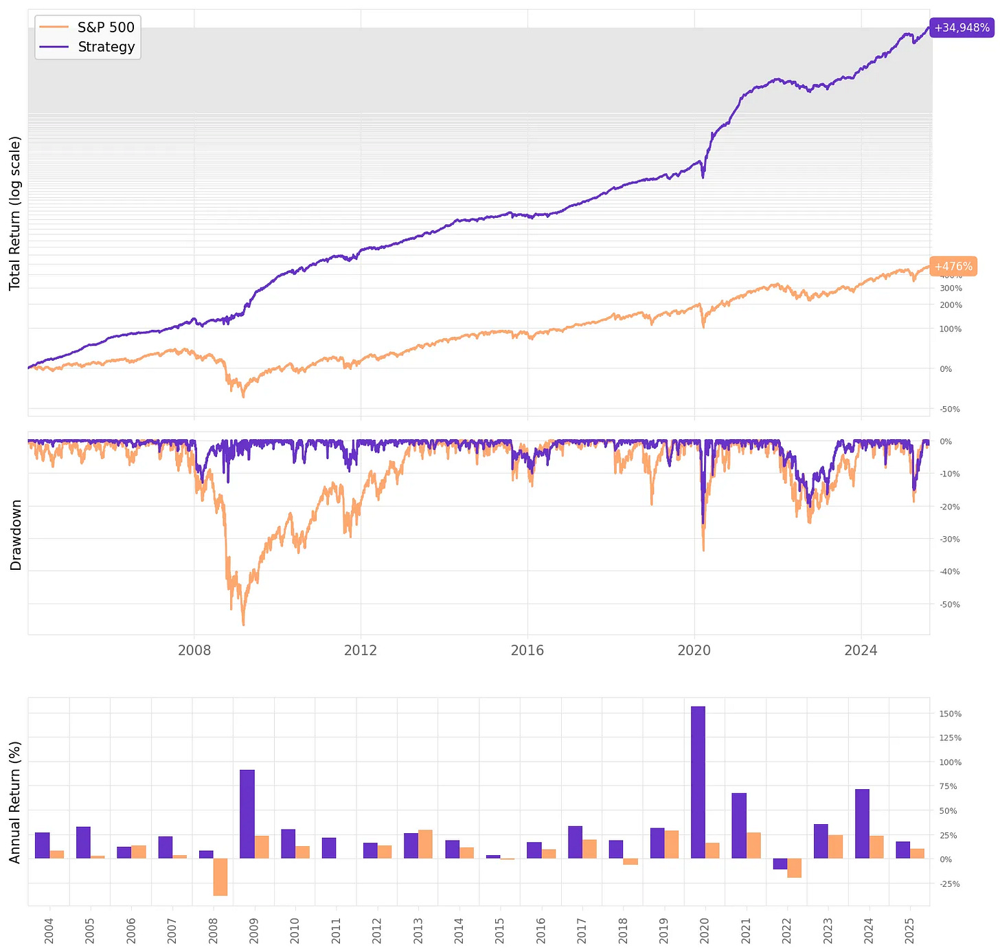
The backtest looks stellar, but only because it relies on two unrealistic assumptions: no trading costs and the ability to buy unlimited size in any stock, regardless of liquidity. Trading costs are not negligible here (especially for a strategy that rebalances every single day), and market impact in less liquid names would quickly eat into performance. The result is an equity curve that looks great on paper but overstates what a tradable strategy could actually deliver.
And that’s not unusual. Academic papers often skip over these implementation details (costs, liquidity, capacity) because their focus is on documenting the signal itself. It’s our job as practitioners to stress-test those assumptions, adjust for reality, and see whether the idea survives outside the lab.
Modeling friction and trading costs
There are many different ways to model friction. As it was famously said:
“All models are wrong, but some are useful.” George E. P. Box.
To bring the strategy closer to reality, we’ll model two critical frictions using the following rules:
Commissions
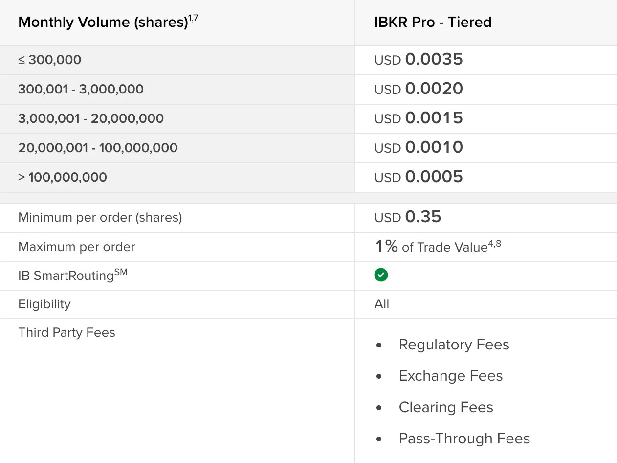
We will implement Interactive Brokers’ tiered model:
Monthly volume shares are computed using the unadjusted closed prices of all names traded
We consider +$0.0020 in third-party fees (approx. 2x the values in every tier)
We will consider these dollar values fixed throughout the simulation (which is a conservative estimate, as these numbers were lower 20 years ago)
Liquidity constraints
If the required order size exceeds 10% of a stock’s daily volume, we assume the trade cannot be executed and skip it entirely.
Together, these adjustments transform the “too good to be true” backtest into something that better reflects what can actually be achieved.
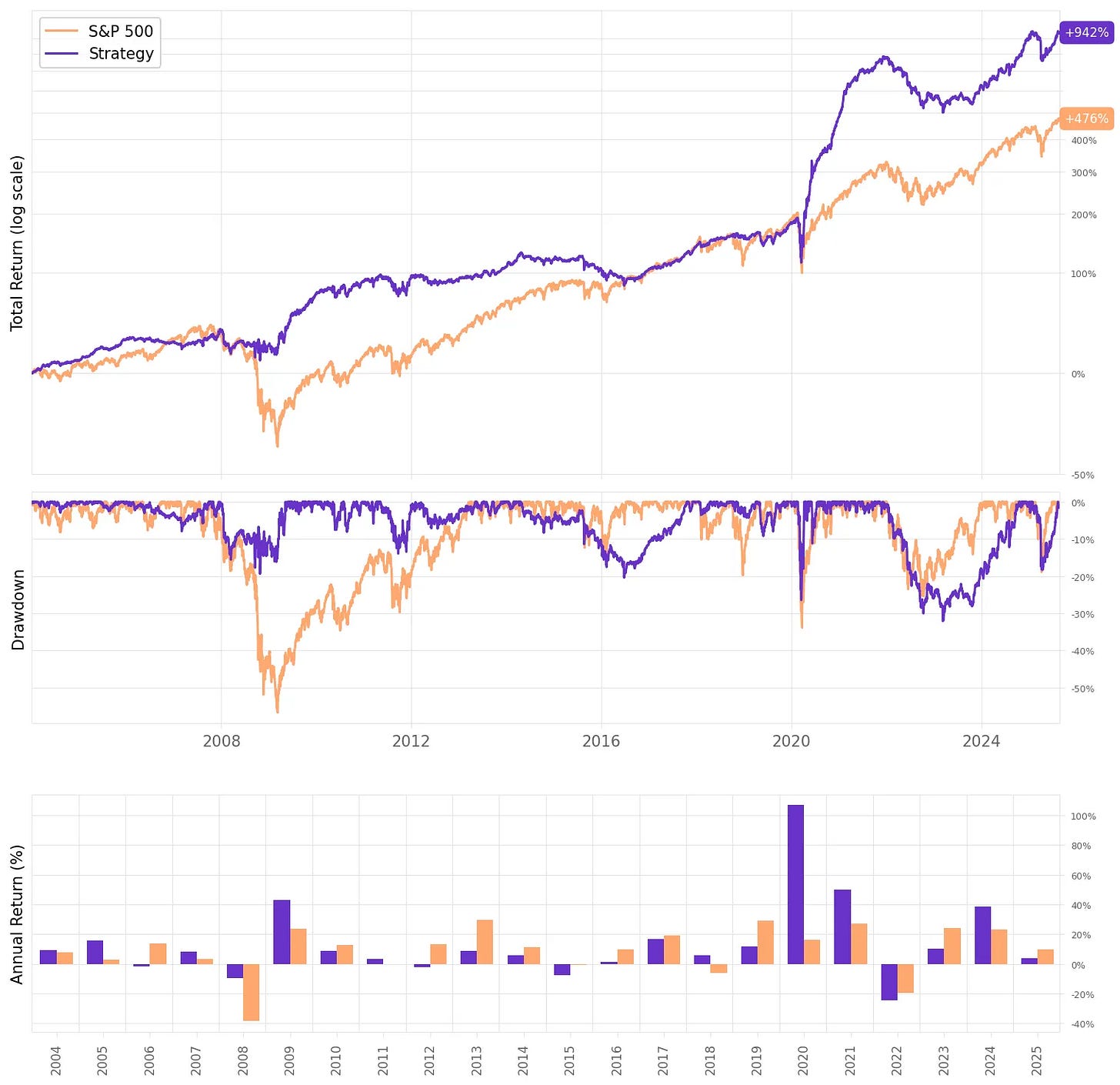
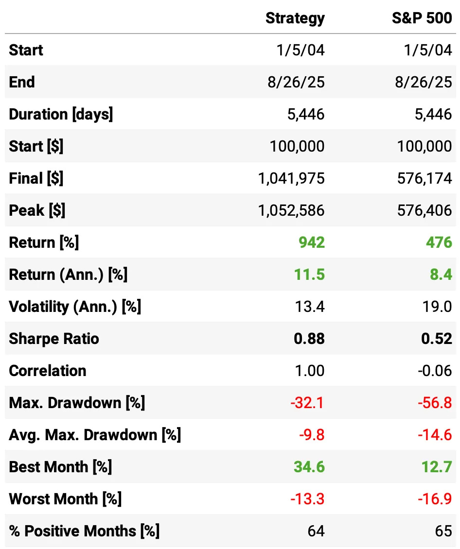
Let's see how they impact the strategy:
With trading costs and liquidity frictions modeled, the picture becomes more realistic. The strategy still outperforms the S&P 500 benchmark in terms of annualized return and Sharpe ratio, proving that the overnight volume-shock effect is economically meaningful. But the performance is nowhere near the “frictionless” backtest, exactly as expected. Once we factor in commissions and the inability to size up in illiquid names, a good chunk of the edge gets eaten away, leaving behind a strategy that doesn't meet our standards to go into production.
What can we do to fix that?
Changing the universe
At this point, many people would throw in the towel. They’d look at the results, dismiss the strategy as untradable, maybe even blame the academics for skipping frictions, and then move on to the next shiny idea. And that’s fair — everyone can do as they please.
But as a fan of Janis Joplin, I prefer to “try, just a little bit harder.”
This strategy is all about overnight returns — and if you’ve spent any time watching the markets, you know there’s a special corner of it that lives and breathes overnight moves: biotech stocks. They’re notorious for sharp gaps up or down, often tied to drug trial results, FDA decisions, or corporate announcements that tend to hit after hours. Big overnight moves, weak intraday drifts — it’s almost textbook for our setup.
Thanks to Norgate data, we have survivorship-bias-free constituents of the Nasdaq Biotechnology Index going back decades. So let’s narrow our focus to that universe and see whether the strategy becomes not just academically interesting, but practically powerful.
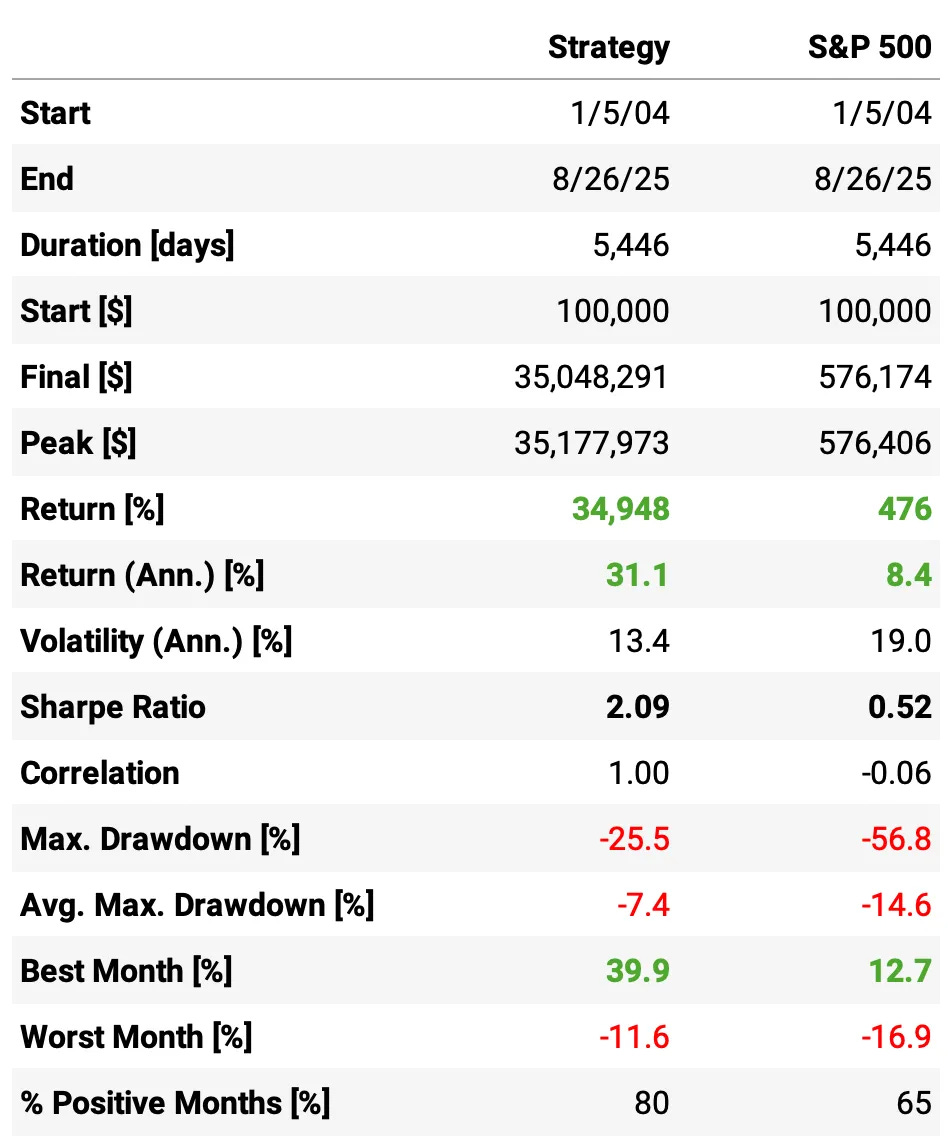
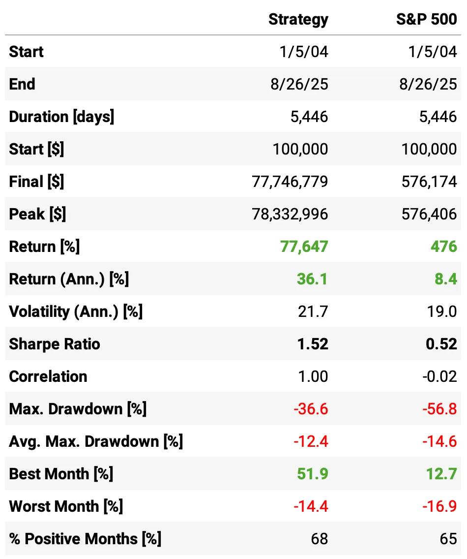
The results are striking:
Annualized return is 36.1%, more than four times the S&P 500’s 8.4%;
Sharpe Ratio is 1.52, nearly three times higher than the benchmark’s 0.52, showing much stronger risk-adjusted performance;
Volatility comes in at 21.7%, slightly higher than the S&P 500’s 19.0%, but well compensated by the excess return;
Maximum drawdown is -36.6%, considerably smaller than the S&P 500’s -56.8% (but still high for most investors);
Correlation to the S&P 500 is effectively zero, offering diversification benefits;
The strategy also delivered 68% positive months, with a best month of +51.9% — versus the benchmark’s +12.7%.
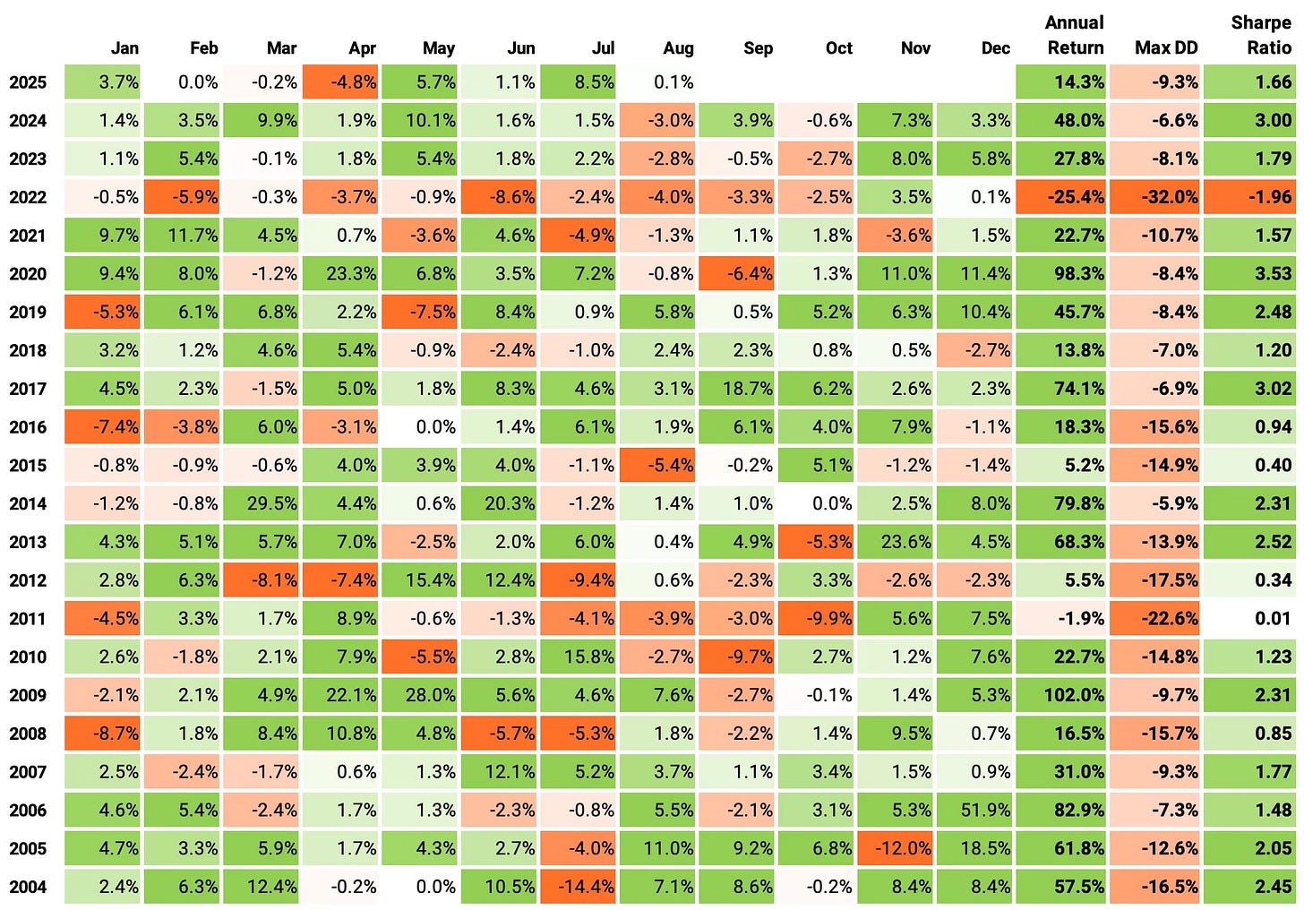
This is the distribution of monthly returns. Here are some interesting highlights after computing the key descriptive statistics measures:
Mean (2.8% per month): That compounds to ~36% annualized, in line with the backtest table. Strong absolute performance.
Std (6.8%): Moderate monthly volatility.
Min (-14.4%) vs. Max (+51.9%): Extreme dispersion. While the downside is capped at about -14%, the upside tails are very fat (a +52% month!), likely driven by biotech gap-ups.
Median (1.9%) vs. Mean (2.8%): Mean > Median indicates the distribution is positively skewed — the occasional explosive winners pull the average up.
Skew (2.1): Strongly right-skewed. This is exactly what you’d hope for in a strategy: more frequent modest gains, with rare huge wins.
Kurtosis (11.6): Very heavy tails compared to a normal distribution (which has kurtosis of 3). This means more extreme outliers — both positive and negative — though the skew suggests the extreme positives dominate.
Final thoughts
As it stands, the strategy is powerful but not for the faint of heart. Volatility runs higher than the benchmark, and while that risk is handsomely rewarded (a 1.5 Sharpe ratio is good), most investors don’t have the stomach for drawdowns north of 15–20%.
How to fix that? The naive solution is simple: don’t deploy all your capital here. Allocate a smaller slice and let the high Sharpe ratio do the compounding work. A second approach is to treat it as a component within a larger portfolio of strategies — its near-zero correlation to the market makes it an attractive diversifier. And of course, we could explore hedging overlays (like the beta hedging framework we discussed in earlier articles) to dampen volatility without giving up much alpha.
And this is only the start. Now that we’ve established a strong baseline, there’s plenty of room to push further. We could train models to predict the sign of the overnight return, using volume shock as a feature but expanding the set with price action, volatility, or news-driven variables. Both linear and non-linear methods could be tested, from simple regressions to richer ML frameworks. In short, the canvas is wide open — there’s much more we can do.
As always, I’d love to hear your thoughts. Feel free to reach out via Twitter or email if you have questions, ideas, or feedback. And if you’re looking to bring a strategy like this into production, let me know — especially if you’re running at scale, where low execution costs can make all the difference.
Cheers!
Course and Community: enrollments Open
As many of you requested, the 2nd cohort of the course is now live and open for enrollment.
It walks through my codebase step by step and is designed for readers who want to develop quant strategies using the same approach I’ve shared here.
You’ll find all the details—content, structure, pricing, and FAQs—at the link below. If you have any questions, feel free to reach out.
Enrollment also includes access to the private community and an ever-growing library of study groups. The code and full recording of the latest session (“Execution details of Intraday Momentum for ES & NQ”) are already available.


Great read—overnight returns have provided a persistent edge for years, and combining that with volume insights adds a powerful dimension. I recently published an article on a systematic volume-based signal for Bitcoin (https://alinakhay.com/p/a-systematic-volume-edge-for-spotting), and it’s fascinating to see how volume-driven signals can deliver predictive power across different markets. Really appreciate your thorough analysis—excellent work!
Just wondering - Why split the data into quantiles if only taking positions in the top 10? Would the pool of stocks not be large enough to take the top ten names (*liquidity dependent) without splitting into quantiles?
Also - The same names in biotech may be used for several days correct? Often large volume shocks are followed by multiple days of large volume
*Sorry new at any of this stuff