Beta hedging
A practical implementation that halves market exposure while preserving alpha


The idea
"If you're not thinking about risk, then you're not thinking." William Sharpe.
William Sharpe is a Nobel Prize-winning economist renowned for his work on the Capital Asset Pricing Model (CAPM) and the Sharpe Ratio, both of which highlight the central role of risk in pricing and evaluating assets. While the quote “If you're not thinking about risk, then you're not thinking” may not be his exact words, it captures the essence of his legacy: that risk must be understood, measured, and deliberately managed.
This week, we’ll show how to systematically hedge a long-biased portfolio of strategies to reduce its market exposure to near zero. It will be a simple yet practical example, with code included. The basic model can be further extended or refined as needed.
Here's the plan:
First, we’ll review a portfolio of strategies, examine its performance, and highlight the issue of having a moderately high beta.
Then, we’ll outline a hedging approach designed to bring the portfolio’s overall beta close to zero.
Next, we’ll run experiments to evaluate how this hedging impacts the portfolio’s overall returns.
Finally, we’ll share some concluding thoughts and discuss possible next steps.
Let's get to it.
As many of you requested, the course is now live and open for enrollment.
It walks through my codebase step by step and is designed for readers who want to develop quant strategies using the same approach I’ve shared here.
You’ll find all the details—content, structure, pricing, and FAQs—at the link below. If you have any questions, feel free to reach out.
Now, to the article!
The problem
We’ve been trading a portfolio of mean reversion strategies—based on ideas we’ve shared here—for over six months. The live results are promising: a return of +10.1% versus -2.8% for the S&P 500. Here’s an overview of the portfolio’s performance:


A portfolio with a 1.1 Sharpe Ratio is what I’d consider OK. Someone asked me over email what I consider a good Sharpe ratio, and here’s the heuristic I use:
< 1.0: Subpar or not investable
1.0–1.5: OK strategy/portfolio
1.5–2.0: Good strategy/portfolio
2.0–3.0: Great strategy/portfolio
> 3.0: Amazing or outlier strategy/portfolio
I always interpret these numbers in the context of capacity. For niche or capacity-constrained strategies, higher Sharpe ratios may be possible—but they’re typically not scalable. Since this portfolio trades only S&P 500 constituents and therefore has very high capacity, a 1.1 Sharpe is reasonable. It's over twice the S&P 500.
The correlation to the S&P 500 is 0.57, which I consider moderately high.
Now, let's use the Fama-French 3-Factor Model to analyze how much of the strategy's performance can be attributed to common risk factors like the market, size, and value. By running an OLS regression on the strategy's excess returns using the Fama-French factors, we can break down the sources of performance into:
Market Risk (Mkt-RF): The sensitivity of the portfolio to market movements, which reflects general market exposure.
Size (SMB): The sensitivity of the portfolio to the size factor, indicating whether it leans towards small or large-cap stocks.
Value (HML): The sensitivity to the value factor, showing whether it favors value or growth stocks.
Here are the results:

The OLS regression on the strategy’s excess returns using Fama-French factors shows a statistically significant alpha of 0.0534, alongside a market beta (Mkt-RF) of 0.57, which is moderately high. Exposure to SMB is small but positive, while the negative HML loading suggests a tilt away from value stocks.
While the positive alpha is encouraging (annualizes to 14.4%), the moderately high beta indicates that a large portion of the returns is explained by general market movements, rather than pure strategy edge. This is not ideal—especially in a multi-strategy or market-neutral framework—because it means the portfolio is still exposed to systematic market risk. Our goal is to hedge this market exposure to isolate the strategy’s true performance and reduce drawdowns during broader market downturns.
This is the problem we are solving. Let's see how.
Beta hedging
Beta hedging is the process of neutralizing a portfolio’s exposure to broad market movements by taking an offsetting position in a market index, typically using futures or ETFs. The goal is to isolate the strategy’s alpha by removing the influence of systematic risk.
In our case, the portfolio has a market beta of 0.57, meaning it tends to move 0.57% for every 1% move in the S&P 500. To offset this exposure, we’ll short S&P 500 futures (ES contracts) in proportion to the portfolio’s beta and current notional value. This allows us to bring the net beta close to zero, reducing sensitivity to market direction.
We’re not attempting to hedge other factors like SMB or HML (their betas are not as high). Our focus here is purely on market exposure. Because beta and portfolio value can fluctuate daily, we’ll recalculate the hedge each day and adjust the number of ES contracts accordingly. This ensures the portfolio stays close to beta-neutral over time.
This is meant to be a simple, focused example to demonstrate the concept. Extending the approach to hedge exposure to other risk factors—such as size (SMB) or value (HML)—follows the same logic: estimate the factor loading, identify a tradable proxy, and size the hedge accordingly.
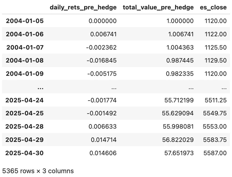
We start with a DataFrame containing three columns:
daily_rets_pre_hedge– the portfolio’s daily returns before applying the hedgetotal_value_pre_hedge– the portfolio’s total dollar value each dayes_close– the daily closing price of the S&P 500 futures (ES)
Now, we need to compute the rolling beta of this portfolio:

The code above estimates the portfolio’s rolling beta to the market using a 63-day window. For each window, it applies the get_alpha_and_betas function to compute the market beta (Mkt-RF), which is then forward-filled to handle any initial NaNs. To smooth short-term fluctuations, the resulting beta series is further filtered using an exponential moving average (EMA) with a 20-day span. Additionally, the portfolio’s daily notional value is scaled to an initial capital of $1,000,000, and rows with missing values are dropped to prepare the data for hedging calculations.
The method get_alpha_and_betas is something like this:

The get_alpha_and_betas function runs an OLS regression of a strategy’s excess returns against the Fama-French factors (either 3 or 5), in order to estimate the strategy’s alpha and factor loadings (betas). It first downloads and preprocesses the relevant factor data using the external helper get_ff_factor_model, which pulls data directly from Kenneth French’s website (https://mba.tuck.dartmouth.edu/pages/faculty/ken.french/) and returns it ready for regression (this helper is included in the course but not shown here for brevity). The strategy returns are joined with the factor dataset, and if there are enough data points (default: 42), a regression is run using statsmodels.OLS.
Then, we can see the rolling beta with the following snippet:


Now that we’ve estimated the portfolio’s rolling beta, we can compute the number of ES contracts to hold each day and track the impact of the hedge on both PnL and overall portfolio returns:
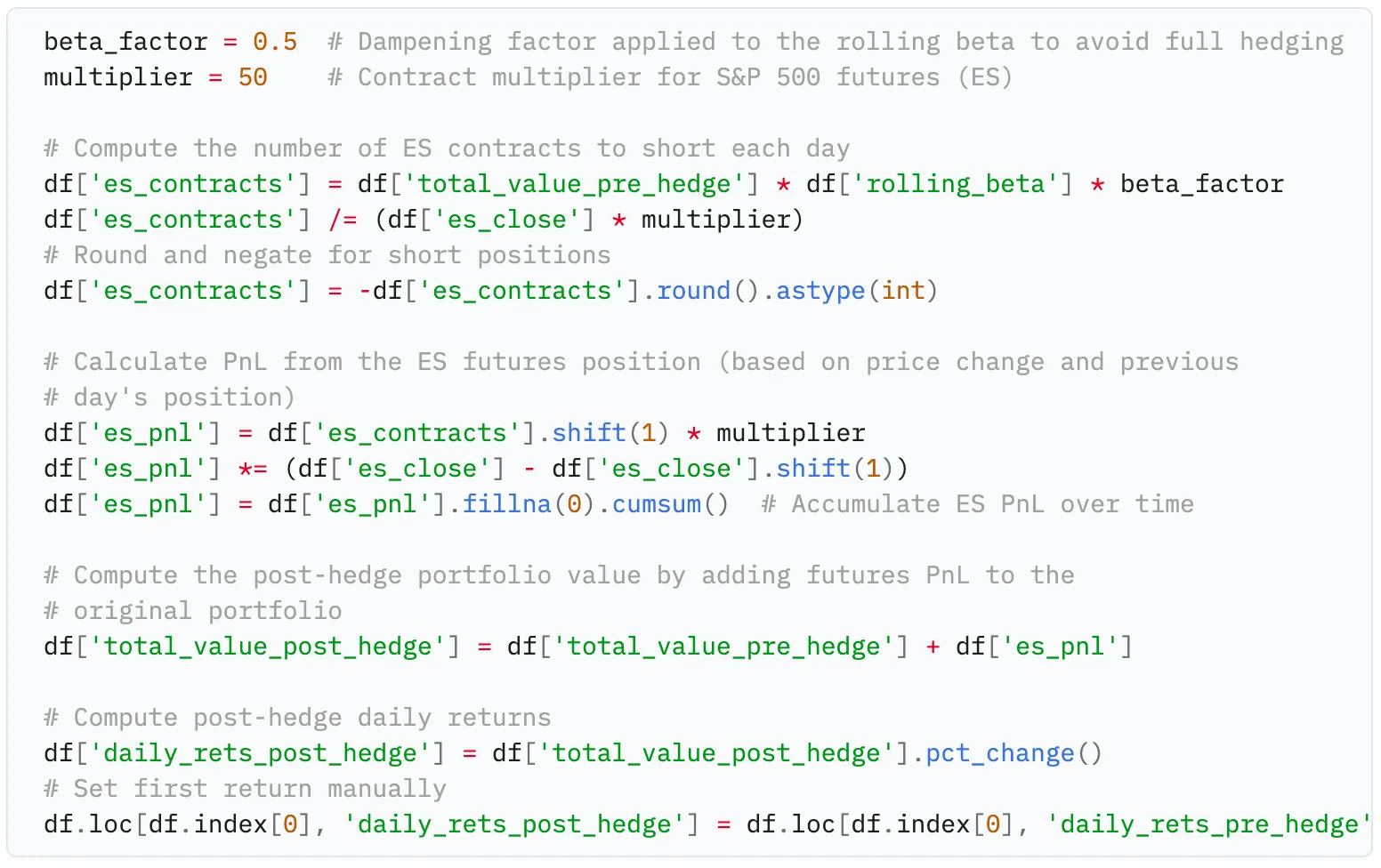
Here's what the code above is doing, step-by-step:
Hedge Sizing:
The number of ES futures contracts to short is calculated based on the portfolio’s dollar value, its rolling beta, and a dampening
beta_factor(set to 0.5). The hedge is not fully sized to neutralize all beta—this allows for some market exposure to remain, which may improve Sharpe or reduce over-hedging. The hedge is scaled by the ES contract multiplier (50), and the result is rounded to an integer and negated to reflect a short position.Futures PnL Calculation:
The PnL from holding the ES futures is computed as the change in futures price multiplied by the previous day’s position size and the contract multiplier. This simulates daily rebalancing, where the position is adjusted at each step based on the updated beta.
Post-Hedge Portfolio Value:
The PnL from the futures hedge is added to the original (pre-hedge) portfolio value to compute the total value of the post-hedge portfolio. This reflects how the hedge offsets market-driven moves in the unhedged portfolio.
Post-Hedge Returns:
Finally, the daily returns of the post-hedge portfolio are calculated as the percentage change in total value. The first day's return is manually set to match the pre-hedge return to avoid a missing value at the start of the series.
Results
Now, we can see the new results:
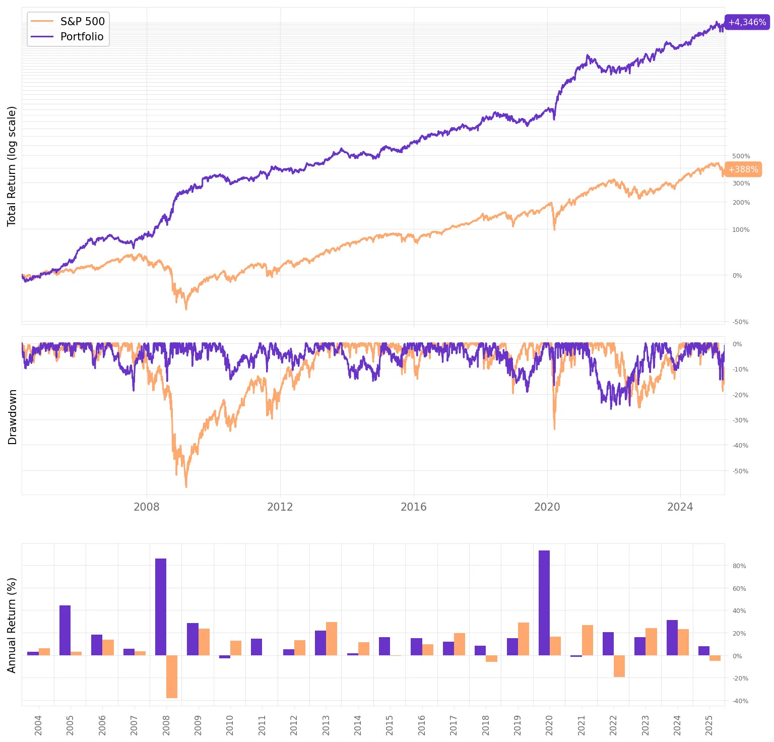


Here are the main highlights and conclusions from the pre- and post-hedge performance comparison:
Market exposure was significantly reduced:
Correlation to the S&P 500 dropped from 0.57 pre-hedge to 0.29 post-hedge, indicating effective removal of systematic market risk.
Sharpe ratio remained stable:
The Sharpe ratio stayed nearly unchanged (1.09 → 1.08), suggesting that the hedge did not dilute the portfolio's risk-adjusted performance.
Return and volatility slightly decreased:
Annualized return decreased marginally (21.0% → 19.8%) along with volatility (19.1% → 18.2%), consistent with a dampened beta.
Max drawdown slightly increased:
Maximum drawdown worsened slightly (-24.4% → -26.0%), which may reflect the cost of daily rebalancing or increased short-term fluctuations introduced by the hedge.
Reduced dependence on market direction:
Despite lower beta, the strategy preserved almost all of its long-term return, which reinforces the presence of true alpha.
Re-running the Fama-French 3-Factor Model allows us to assess how much of the strategy’s performance can be explained by common risk factors. The results are as follows:

Highlights:
Market beta dropped substantially:
The loading on Mkt-RF fell from 0.57 pre-hedge to 0.27 post-hedge, confirming that the hedge significantly reduced market exposure.
Alpha increased after hedging:
The annualized alpha rose from 14.4% to 16.4%, suggesting that isolating the portfolio from market movements revealed even stronger idiosyncratic performance.
Model explanatory power decreased:
The R-squared dropped from 0.33 to 0.09, indicating that a much smaller portion of the portfolio’s returns is now explained by the Fama-French factors—consistent with a more market-neutral profile.
Alpha remained statistically significant in both cases (p-value < 0.001), reinforcing the robustness of the strategy’s non-factor-driven edge.
These results validate that the hedge effectively reduced systematic risk while preserving the portfolio’s alpha characteristics.
To wrap up the analysis, the chart below offers a visual comparison of the portfolio’s daily returns versus the S&P 500 before and after hedging:

The left panel shows a clear positive relationship between the portfolio and the market, with a beta of approximately 0.57. After applying the hedge (right panel), the slope of the linear fit drops to 0.27, confirming that the portfolio’s sensitivity to market movements has been significantly reduced. The post-hedge cloud is more centered and less tilted, illustrating how the hedge successfully dampened systematic exposure while retaining the core return profile.
Final thoughts
This was a simple but effective demonstration of how to implement beta hedging in practice. Starting from a long-biased portfolio of strategies with a moderately high market beta, we systematically reduced its exposure by shorting S&P 500 futures, recalibrating the hedge daily. The results were encouraging: we cut the beta nearly in half, maintained the Sharpe ratio, and preserved nearly all of the original alpha—while significantly lowering the portfolio's correlation to the market.
While the model we used was intentionally simple, the core concept generalizes well. Hedging other factor exposures—such as size or value—follows the exact same playbook. The point wasn’t to overfit, but to show that a practical, transparent beta hedge can be built with just a few lines of code and some clean assumptions.
There’s room to explore further. One direction is to turn this static hedge into a more dynamic framework, where the dampening factor or even the hedge asset itself adjusts based on regime shifts or higher-order factor interactions. Another is to combine beta hedging with volatility targeting or cross-asset overlays to create a fully adaptive market-neutral engine.
But that’s a topic for another day.
As always, I’d love to hear your thoughts. Feel free to reach out via Twitter or email if you have questions, ideas, or feedback.
Cheers!
As many of you requested, the course is now live and open for enrollment.
It walks through my codebase step by step and is designed for readers who want to develop quant strategies using the same approach I’ve shared here.
You’ll find all the details—content, structure, pricing, and FAQs—at the link below. If you have any questions, feel free to reach out.