From Defense to Offense: A Tactical Model for All Seasons
How to get a +1.40 Sharpe ratio from adjusting a simple TAA model


The idea
“Basketball is a game of adjustments.” Bob Knight.
Bob Knight was the last coach to lead an NCAA team to a perfect season: 32 wins, zero losses. That record still stands nearly half a century later.
His secret? He was a masterful tactician. Obsessed with preparation, relentless on fundamentals, and unmatched in making in-game adjustments. Knight believed basketball wasn’t about memorizing plays, but about reading the moment and adapting faster than the opponent. This philosophy made him one of the greatest coaches of all time.
This week, we will implement the idea from the paper Defense First: A Multi-Asset Tactical Model for Adaptive Downside Protection, by Thomas Carlson (2025). (You can find more about Tom here: Tom Carlson.)
Tactical Asset Allocation (TAA) takes the same principle of adaptability and applies it to investing. While Strategic Asset Allocation sets a long-term baseline mix (e.g., 60% stocks, 40% bonds), TAA introduces short- to medium-term adjustments based on market conditions. The goal? Exploit opportunities or mitigate risk by shifting weights dynamically, adding offense in favorable environments and defense when risks rise.
Lately, I’ve leaned toward more advanced ideas, which might explain why so many readers are now coming from places like Morgan Stanley, Goldman Sachs, Deutsche Bank, Citigroup, Millennium Management, Point72, Wellington Management, Man Group, Millburn, Trexquant, IMC Trading… to name a few. (As well as students from schools like MIT, Columbia, Cornell, UPenn/Wharton, Carnegie Mellon, Duke, NYU, Berkeley, Georgia Tech, Imperial College London, etc.)
That said, I often get requests to cover simple ideas. This week’s idea is exactly that… so simple that you can code it in under 40 lines.
Here's our plan:
First, we will summarize the paper
Then, we will discuss why it works and verify the edge quantitatively
Next, we will improve the original idea
Finally, we will discuss next steps
Let's get to it.
Study Group
Our next session will be on Saturday, August 9th at 11 AM ET (33% of the votes) and will focus on execution details from the Intraday Momentum for ES & NQ article (57% of the votes). Connection details will be available at connect.quantitativo.com.
We’re building a private community for systematic traders. A place to explore ideas, exchange insights, and tackle the real technical and strategic challenges of building robust trading systems… from signal research to execution and risk.
Enrollment reopens in August. Join the waitlist below to be the first to know when new seats open:
Paper Summary
Traditional “safe haven” strategies often fail during crises because correlations rise and static allocations break down. Defense First introduces a rules-based Tactical Asset Allocation model that dynamically rotates among four defensive assets—long-term U.S. Treasuries (TLT), gold (GLD), commodities (DBC), and the U.S. dollar (UUP)—with U.S. equities (SPY) as a fallback when defenses weaken. The objective: adaptive downside protection with positive long-term returns.
How It Works
Each month, the strategy ranks four defensive assets based on multi-timeframe momentum (1, 3, 6, 12 months):
TLT (Long-term Treasuries) — deflation hedge
GLD (Gold) — monetary instability hedge
DBC (Commodities) — inflation hedge
UUP (USD Index) — liquidity crisis hedge
Allocations are 40/30/20/10 across the ranked assets if they outperform cash (T-bills). Assets that fail this screen are replaced with SPY (U.S. equities) as a fallback (not for growth, but as the “least weak” option).
It significantly reduced drawdowns during every major crash (1987, GFC, COVID, 2022), and generated 65% profitable months across decades.
Why It Works
Multi-Asset Defense: Each asset hedges a different macro risk (deflation, inflation, currency stress, monetary instability).
Momentum Edge: Builds on well-documented trend persistence across asset classes.
Adaptive Risk Control: Absolute momentum filter avoids weak assets; equity fallback prevents idle cash.
Practical Perks
All instruments are liquid ETFs.
Simple monthly rebalancing.
No reliance on exotic data or proprietary tools.
Easily scalable for institutional or retail portfolios.
The Edge
Before running full backtests, let’s first examine whether the signal has a real edge. There are two ways to do this.
First, we can observe the edge by looking at the average next-month return of assets ranked by their momentum score. Each month, we rank the four defensive assets from 1 (highest momentum) to 4 (lowest momentum), then compute the average return for the following month.
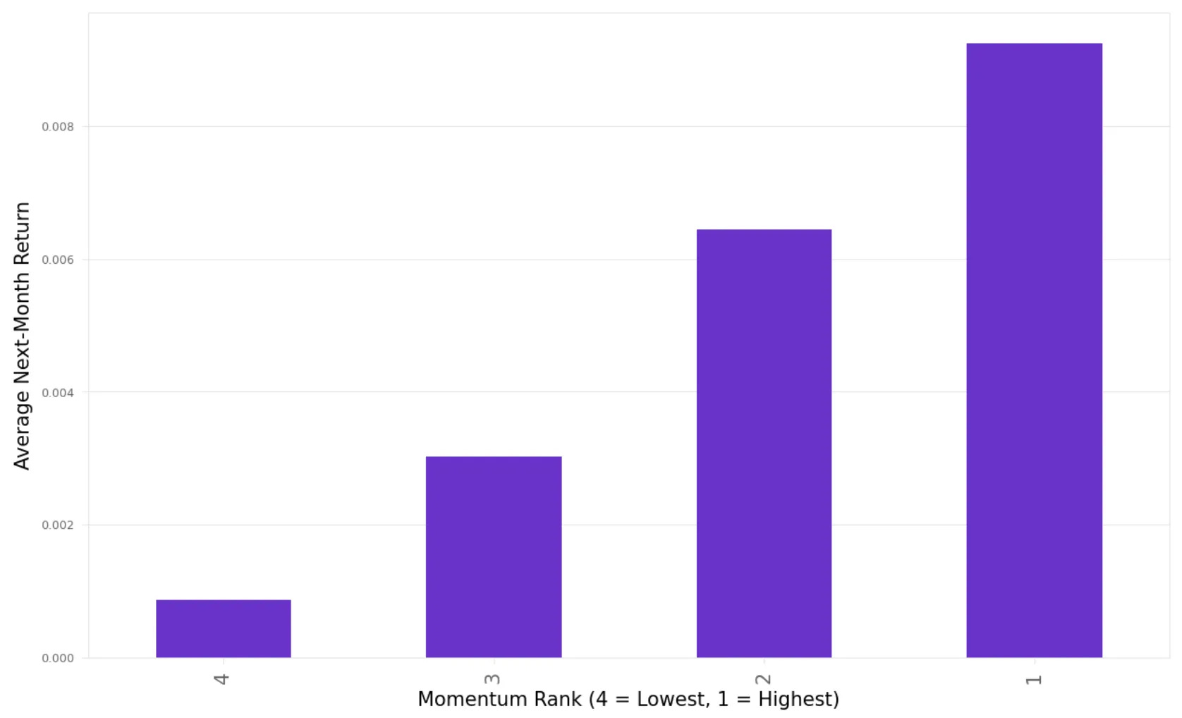
When we average this across 34 years of data, the relationship is clear:
Rank 4 (weakest momentum) delivers the lowest next-month return,
Rank 1 (strongest momentum) delivers the highest,
and the increase is monotonic from left to right.
This means momentum isn’t just a theory here: it shows up in the numbers.
The second way is through a Fama-MacBeth regression, a standard approach in asset pricing to test if a characteristic predicts future returns across assets and time.
Here’s how it works:
Each month, we run a cross-sectional regression of next month’s return on the momentum score for the four defensive assets.
We then average the slopes across all months and compute robust standard errors (Newey-West) to account for autocorrelation.
The result?
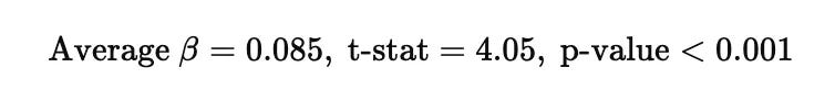
This means that a one-unit increase in the momentum score is associated with an 8.5% higher next-month return on average. Statistically significant at the 1% level, this confirms that the momentum ranking carries real predictive power.
Experiments
Wherever possible, ETF data was used. For periods prior to ETF inception, we filled the gaps with Vanguard mutual funds, asset class indices, or futures proxies, mirroring the methodology in the paper. This approach provides a consistent return history from early 1990s through 2025.
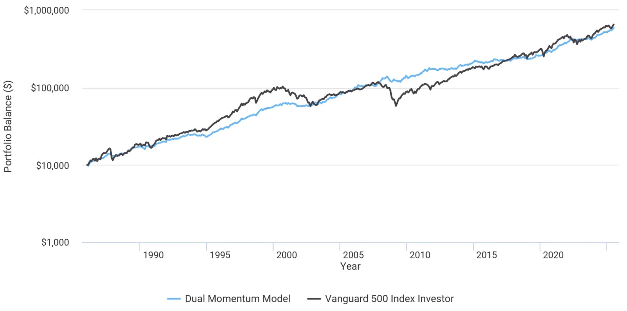
Here’s what the backtest looks like when we implement the strategy exactly as described in the paper:
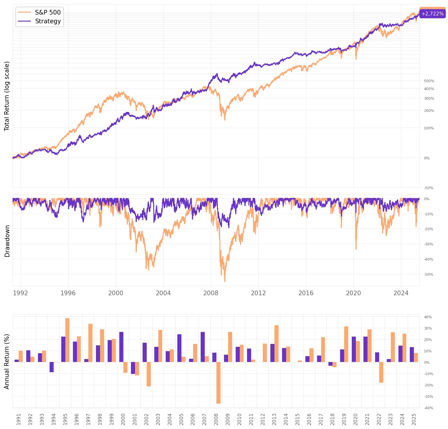
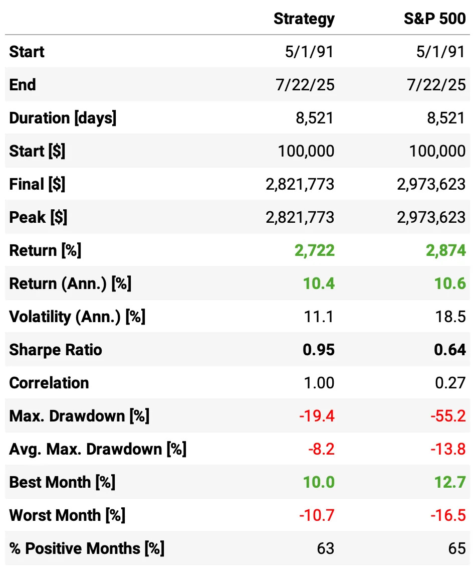
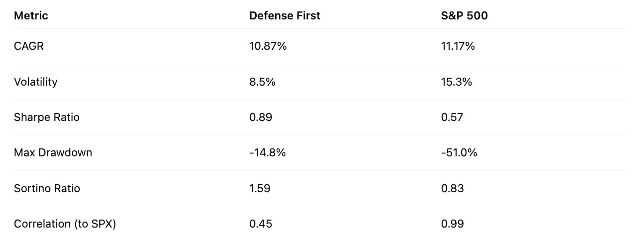
The results are not bad:
Annualized return is 10.4%, very close to the S&P 500’s 10.6%, but with much lower risk;
Sharpe Ratio is 0.95, 50% higher than the benchmark’s 0.64, signaling far better risk-adjusted performance;
Volatility is just 11.1% vs. 18.5% for the benchmark, a significant reduction;
Maximum drawdown is only 19.4%, compared to a crushing 55.2% for the S&P 500;
Correlation to equities is modest at 0.27, adding diversification benefits;
The results are also pretty close to what was presented in the paper.
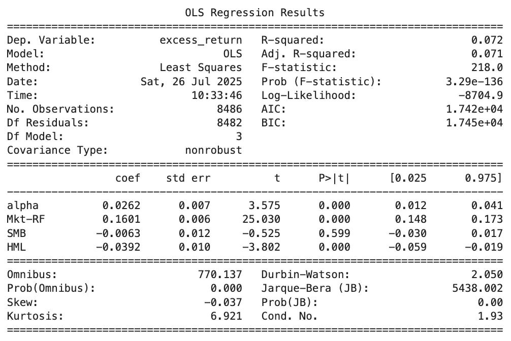
And here are the key takeaways from the Fama-French 3-Factor regression:
Alpha: 0.0262% per day → annualized ≈ 6.8%, statistically significant (t = 3.58, p < 0.001), confirming strong abnormal returns not explained by Fama-French factors;
Market Beta (Mkt-RF): 0.16 → very low equity exposure, yet strong absolute returns;
SMB (Size): -0.006, not significant → no clear size tilt;
HML (Value): -0.039, significant negative → slight tilt toward growth;
R²: 0.072 → factors explain only ~7% of variance, most return comes from strategy itself.
So, the system works: we see a good downside protection.
Now, what can we do to improve the system and go from defense to offense?
Adding leverage
The first idea is simple: add leverage… but not across the board. We’ll apply 3x leverage only to the equity portion by using the UPRO ETF. Why 3x? Because it brings the portfolio’s risk closer to that of the benchmark. See:
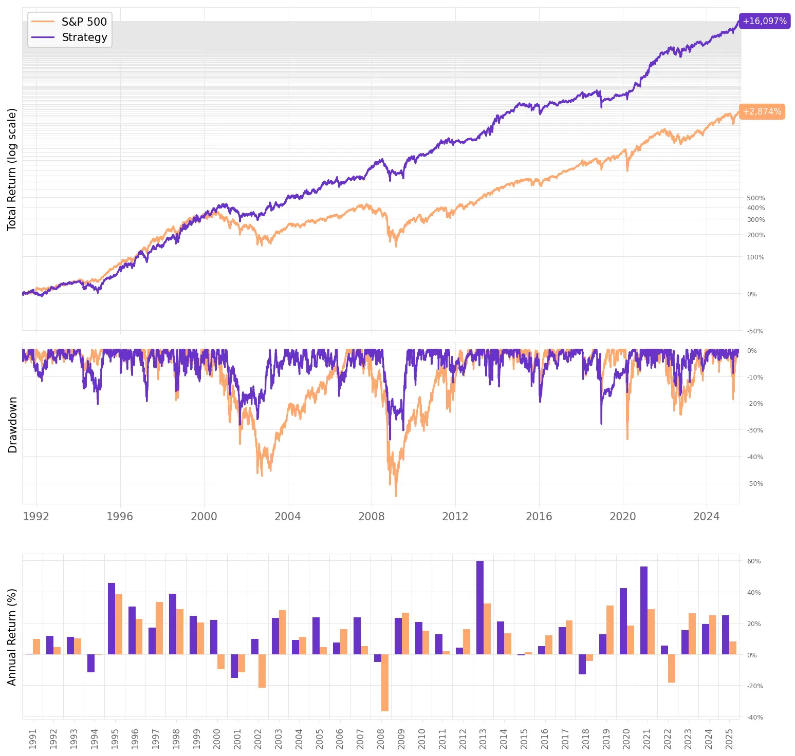
In summary:
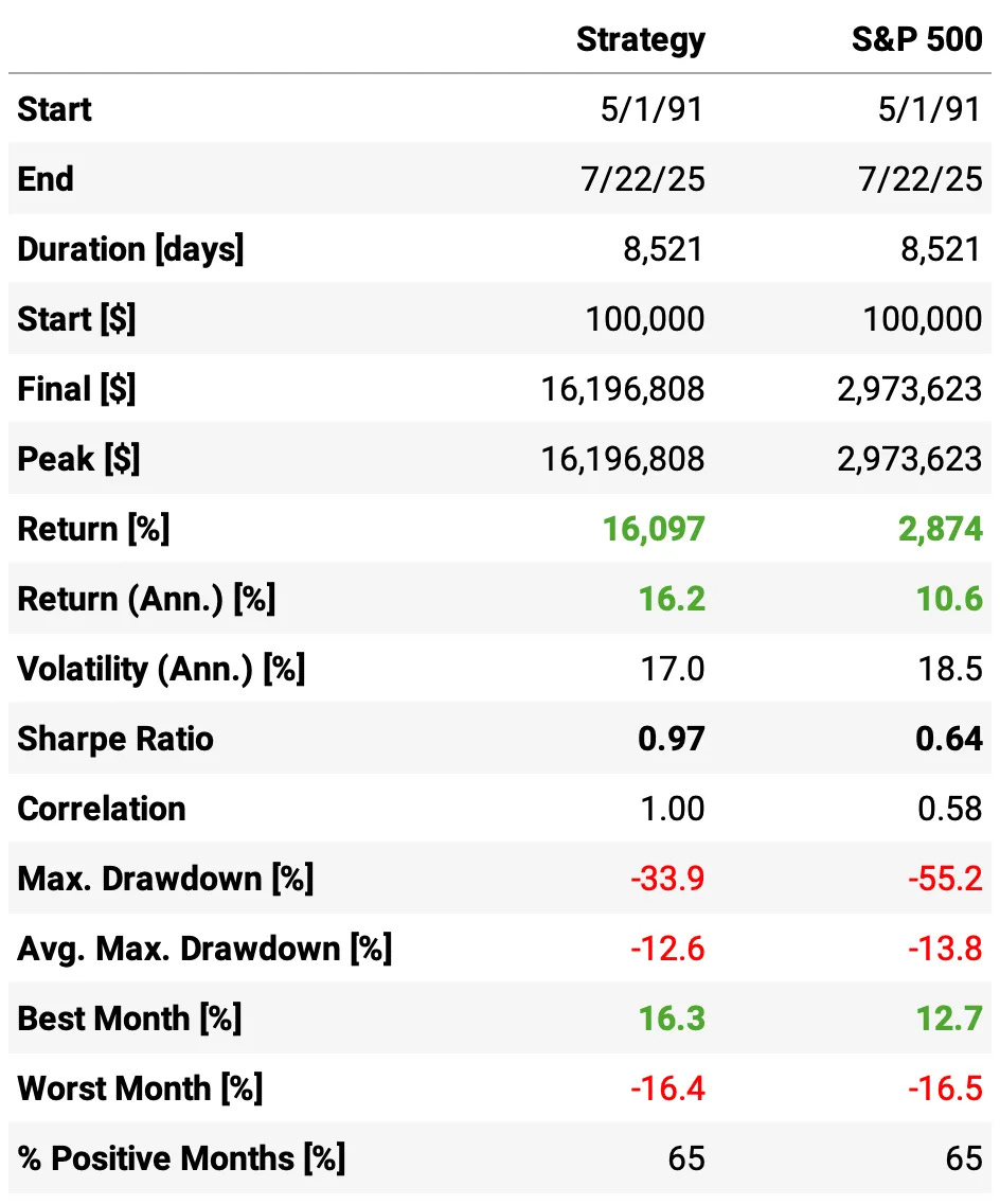
Annualized return jumps to 16.2%, a big increase from 10.4% in the unleveraged strategy, and far ahead of the S&P 500’s 10.6%;
Sharpe Ratio remains good at 0.97, slightly above 0.95 from before, and still much better than the S&P 500’s 0.64;
Volatility rises to 17.0%, up from 11.1%, but still slightly below the S&P 500’s 18.5%;
Max drawdown increases to -33.9%, compared to -19.4% before, but it’s still significantly better than the S&P 500’s -55.2%;
Average max drawdown remains controlled at -12.6% vs. -13.8% for the S&P 500;
Correlation with the S&P 500 rises to 0.58, which is expected since we’ve leveraged the equity sleeve;
With roughly the same level of volatility as the S&P 500, the strategy now delivers significantly higher returns (16.2% vs. 10.6%) while maintaining a superior Sharpe ratio and much smaller drawdowns.
What else can we do to improve?
Portfolio of Strategies
The idea here is simple: add this strategy to a broader portfolio. Which portfolio? For example: 40% this strategy, 40% the rebalancing strategy we reviewed in the previous article, and 20% our classic mean-reversion portfolio.
This is what we get:
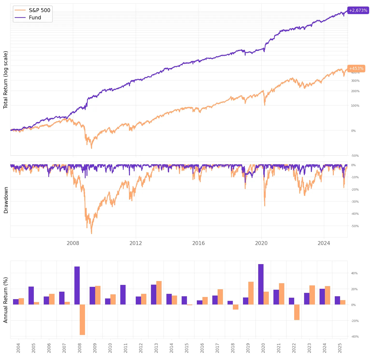
Those results are not bad at all:
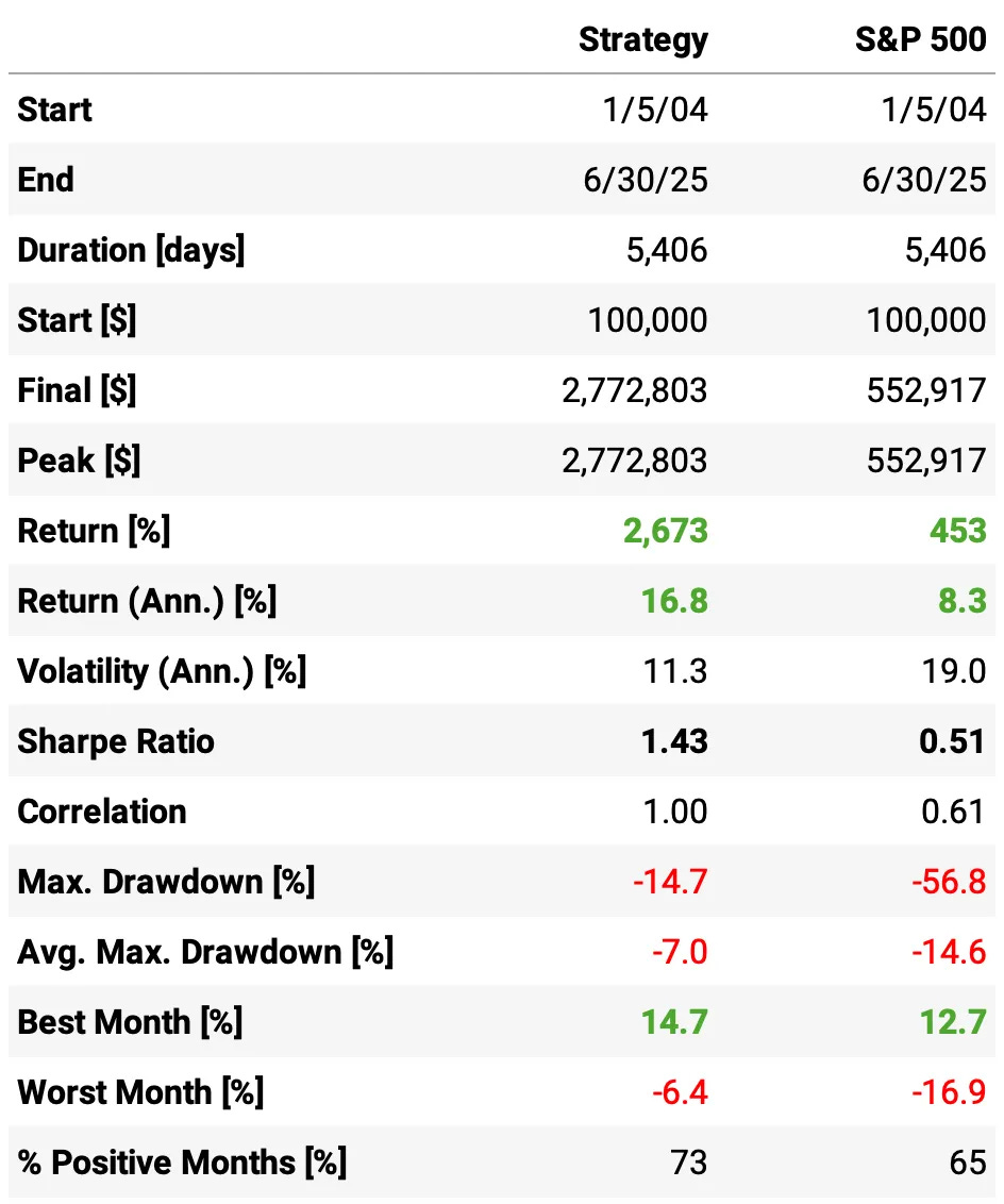
Annualized return climbs to 16.8%, slightly higher than the leveraged version (16.2%) and double the S&P 500’s 8.3%;
Sharpe Ratio jumps to 1.43, a huge improvement over 0.97 in the leveraged strategy and nearly 3x better than the S&P 500’s 0.51;
Volatility drops to 11.3%, far below both the leveraged version (17.0%) and the S&P 500 (19.0%), showing the power of diversification;
Max drawdown improves dramatically to -14.7%, from -33.9% with leverage and -56.8% for the S&P 500;
Average max drawdown shrinks to -7.0%, about half the S&P 500’s -14.6%;
% of positive months rises to 73%, higher than both previous setups (65%) and the benchmark (65%);
Best and worst month performance also improves, with the worst month limited to -6.4% vs. -16.9% for the S&P 500.
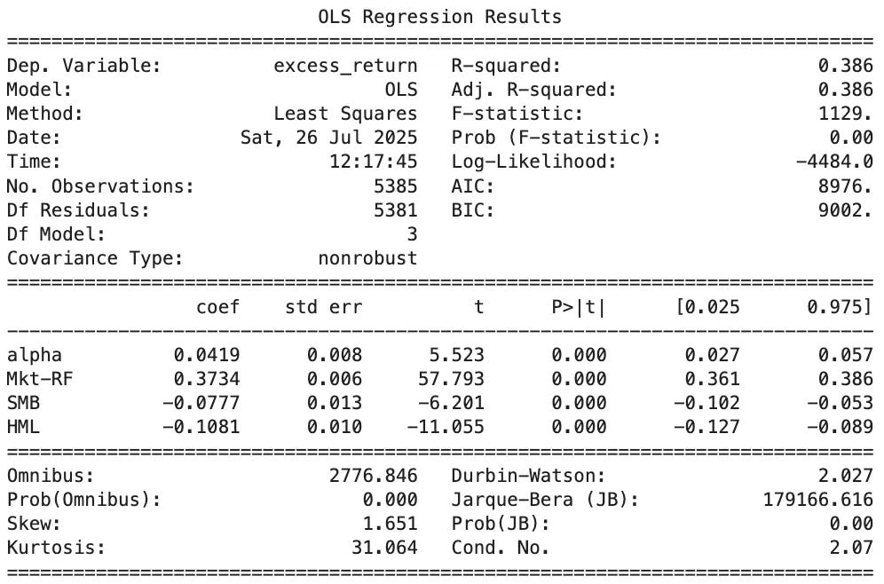
Here are the key takeaways from this Fama-French 3-Factor regression:
Alpha: 0.0419% per day → annualized ≈ 11.1%, highly significant (t = 5.52, p < 0.001), confirming strong abnormal returns unexplained by the factors;
Market Beta (Mkt-RF): 0.37 → moderate equity exposure, much higher than the previous strategy’s 0.16 but still well below 1, meaning returns are not just market-driven;
SMB (Size): -0.078, significant negative → tilt toward large-cap assets;
HML (Value): -0.108, strongly significant negative → strong preference for growth over value;
R²: 0.386 → about 39% of variance explained by the model, leaving most performance driven by the strategy’s design.
Final Thoughts
What started as a defensive allocation model turned out to be a remarkably flexible building block. Out of the box, it offered equity-like returns with bond-like drawdowns, proving that simple rules (momentum screens, absolute thresholds, and macro diversification) can go a long way.
Then we pushed it further. By adding selective leverage, we matched the benchmark’s volatility and delivered a massive return boost without losing control of risk. Finally, by blending this strategy into a portfolio with others, we unlocked more alpha: a 1.43 Sharpe ratio, lower drawdowns, and over 70% positive months.
Does this mean the work is done? Not at all. There’s plenty of room to explore:
Smarter leverage: dynamic sizing based on volatility or market regimes;
Expanded asset set: more macro hedges, or even crypto for an uncorrelated sleeve;
Adaptive weights: machine-learning or Bayesian methods for ranking confidence.
The takeaway? Defense First might be more than a crash-protection tool: a foundation for building robust, adaptive portfolios that thrive across regimes.
As always, I’d love to hear your thoughts. Feel free to reach out via Twitter or email if you have questions, ideas, or feedback.
Cheers!
The first cohort of the course was a great success. Thank you to everyone who joined! Enrollment is now closed. The next cohort opens in August, with 50 more seats. Course participants also get exclusive access to our Community and Study Group. Join the waitlist below to be notified when enrollment reopens:
(I know, I need to update this landing page… as soon as I find time I will add more details about the course, the community, reviews from the 50 first users, etc :))
I had also played around with the leverage while creating this and was pleasantly surprised. I only had from 2005-fwd on PV, but QLD was in kind of a 'sweet spot' for this period (I'm guessing 2002 would not have been as kind ;) LINK: https://tinyurl.com/7h3syxmr
Thanks for this article.. i found it quite interesting.. i thought the world of TAA had been well explored but this was unique. I built my own backtest and review here and of course referenced your post :) https://notfinancial.substack.com/p/defense-first-when-not-losing-is