Murphy's Law
How a fragile mean-reversion idea became a +1.2 Sharpe strategy


The idea
“Anything that can go wrong, will go wrong.”
— Major Edward A. Murphy Jr., aerospace engineer
A few days ago in Abu Dhabi, I met an old friend I hadn’t seen since our graduation. We were among the very few aerospace engineers trained in our home country that year. After a few years serving in the Air Force (I went straight into civilian life, he didn’t), he eventually moved on: first into quantitative hedge funds, and later back into hardcore engineering — his true passion. Today, he’s developing defense drones in the UAE.
“Why do aerospace engineers adapt well to quantitative hedge funds?” one of us asked.
For an airplane to fly, it isn’t enough to get one or two big things right: you need a thousand details to line up. A quantitative strategy is no different: profitability comes from getting a thousand details right. We settled on this hypothesis (five years of nonstop hardcore math and coding might have helped a bit, too :)).
Last week reminded me of one of the most famous aerospace engineers: Major Edward A. Murphy Jr. The man built safety-critical systems… and gifted the world the immortal line (which later became Murphy’s Law), “Anything that can go wrong, will go wrong.” One of the first strategies I wrote about here decided to take that literally — November was brutal for it.
Many people mistake him for a cosmic pessimist or a fatalist. But when he taught his students, “If something can go wrong, it will,” he meant that you should identify everything that could go wrong and fix it so that nothing does go wrong.
This week, instead of dissecting yet another research paper (my last three implementations were so far off from what the authors claimed that I’m starting to wonder who is writing these papers…), let’s talk about how to fix a strategy by getting a thousand details right. Well, maybe not a thousand, but certainly more than a few.
Here’s the plan:
A quick review of the base strategy and a look at what went wrong
A tour through the “more-than-a-few” improvements
Results — because that’s what matters in the end
And as always, a few closing thoughts and the next steps
Let’s get to it.
Study Group
Our last study group was a success. Thank you to all community members who joined live! For those who couldn’t, I will post the code and the recording on learn.quantitativo.com, as usual, in the next few days. The TAA strategy we reviewed is up almost 40% this year.
Lately, our community has shown interest in a wide range of topics on the forum. As usual, I’ll post a survey on connect.quantitativo.com so everyone can vote on the topic for the next study group.
I know I said I would reopen enrollments in December… but I am completely swamped with work, so I’ll reopen enrollments in January 2026. The waitlist already has a few hundred people. Join it below to be the first to know when new seats open:
What is wrong with this strategy
The strategy we’re about to improve is the one described in the article A Mean Reversion Strategy from First Principles Thinking (using only the long-only version for simplicity).
The idea is straightforward: the strategy aims to capture short-term price dislocations in S&P 500 constituents. Whenever a stock experiences a drop that is statistically unlikely (below a certain quantile of its own 5-year return distribution), we open a long position. The trade is closed once the stock reverts.
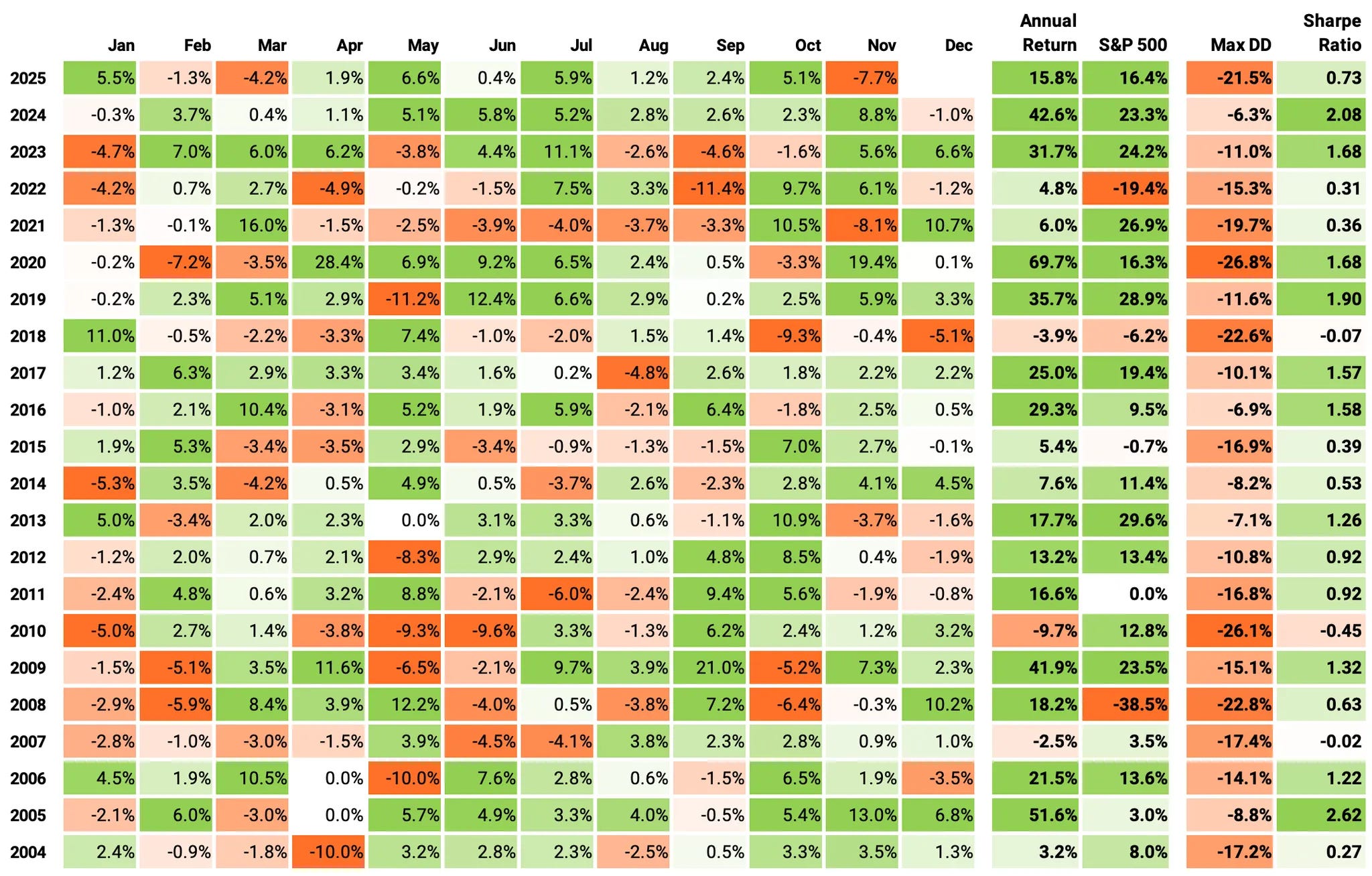
Here’s the performance of the backtest + live since November last year, up-to-date:
Even at first glance, the strategy has several undesirable characteristics:
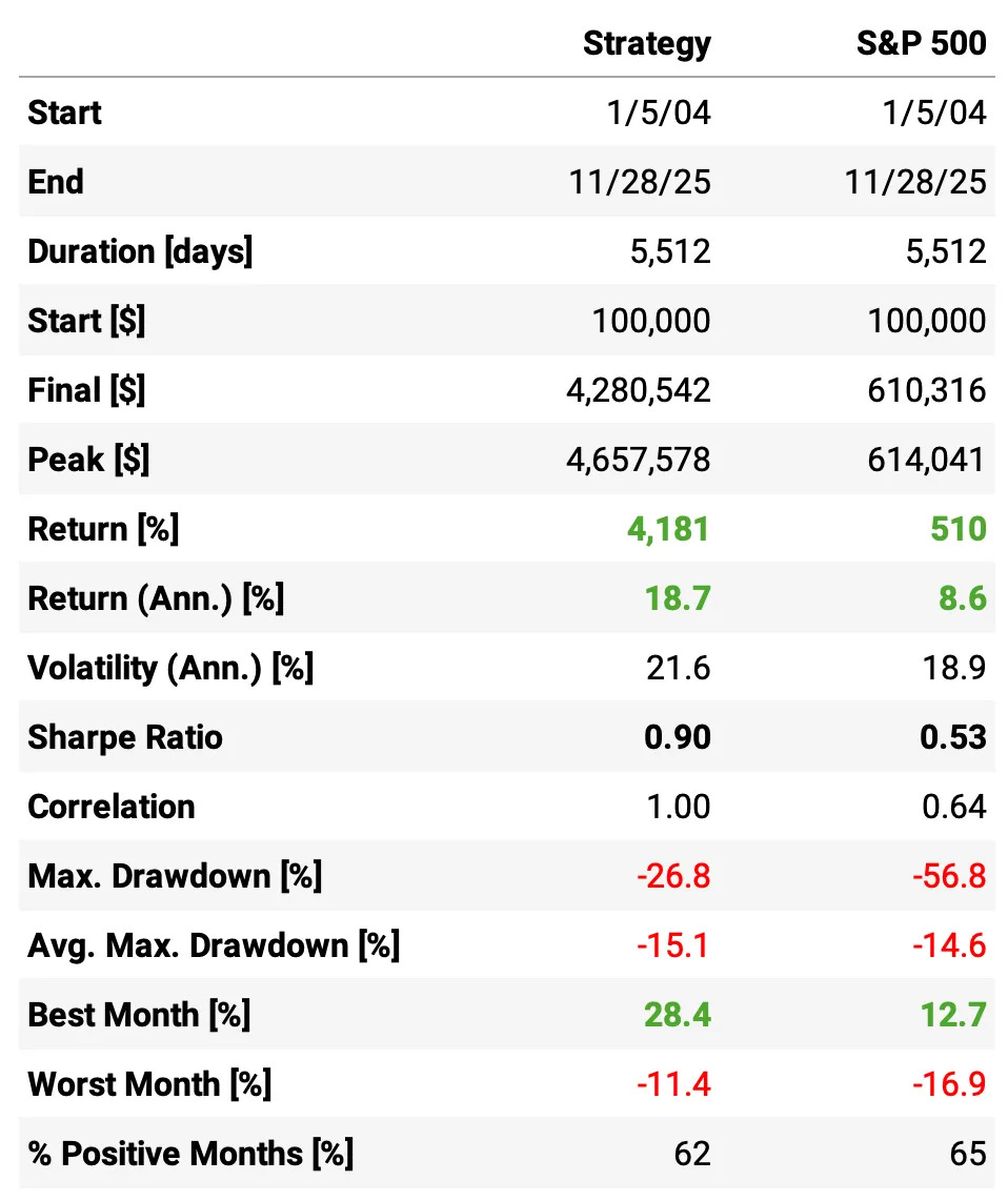
Yes, it outperforms the S&P 500, but the Sharpe ratio isn’t even 1.0
The maximum drawdown is less than half of the benchmark, but at 27% it’s still too high
The average annual drawdown is 15.1% — actually higher than the S&P 500’s 14.6%
The strategy’s volatility is 21.6%, higher than the benchmark
The strategy has a high correlation to the market at 0.64
And November was rough: the strategy returned –7.7% while the market was essentially flat.
Why did this happen in November?
Looking at the individual trades, several were AI-related names (AMD -13%, DELL -12%, ORCL -9%). With only ~20 trades in November, these outsized losses dominated the month’s results.
It’s important to remember that this strategy is designed to profit from short-term statistical dislocations. When a stock undergoes a fundamental repricing, the signal may not mean-revert — because the price change is justified. The system cannot distinguish between:
i) non-fundamental dislocations, and
ii) fundamentally-driven moves.
It captures all statistically significant drops, regardless of their cause.
In November, we saw an unusually high share of fundamental-driven declines, which explains the deviation in performance.
What can we do to fix?
In essence, there are four levers we can pull:
Signal quality → Improve predictive power by separating noise-driven drops from fundamental repricings
Execution logic → Sharpen timing, sizing, and exit rules
Breadth / Diversification → Increase the number of independent bets (more slots)
Risk overlay → Hedge unwanted factor exposures (β, size, momentum, sector, etc.)
In this article, we will focus primarily on (1) and (2). We’ll go deeper on (1), and address (3) and (4) in subsequent pieces. Our goal is to reach a Sharpe ratio of at least 1.5 and cut the maximum drawdown in half.
Improving the edge
A) Baseline
Let’s start by improving the edge — and for that, we need a baseline to compare our experiments against. What would have happened if we had simply bought every event where a stock had:
a price drop,
a 3-day QPI below 15,
a closing price above its 200-day simple moving average (i.e., the stock was in an uptrend),
and then held the position for 5 days?
This is exactly how we measured the edge in the original article. Here are the stats:
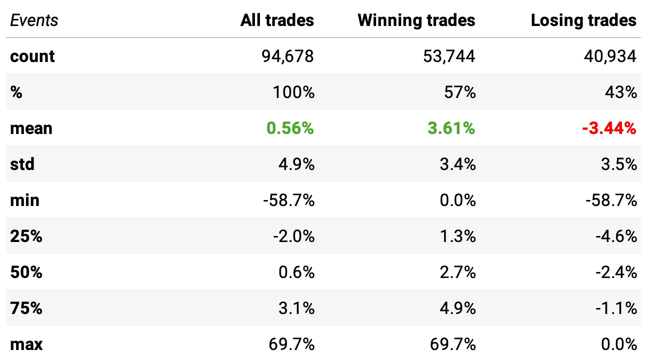
In summary:
Win rate: 57% of the ~95,000 trades were winners (the sample includes only S&P 500 constituents at each point in time to avoid survivorship bias).
Expected return per trade: +0.56% overall (winners averaged +3.6%, losers averaged –3.4%).
Distribution: The median trade was +0.6%, with fairly balanced upside/downside tails (max +69.7%, min –58.7%).
B) Trading at the close
The first improvement was actually proposed by someone in the community a while ago: entering trades at the close instead of at the next day’s open.
This can make sense because many mean-reversion signals are strongest at the moment of the dislocation. By the next morning, part of the move may have already reverted, reducing the available edge. Here’s the data:
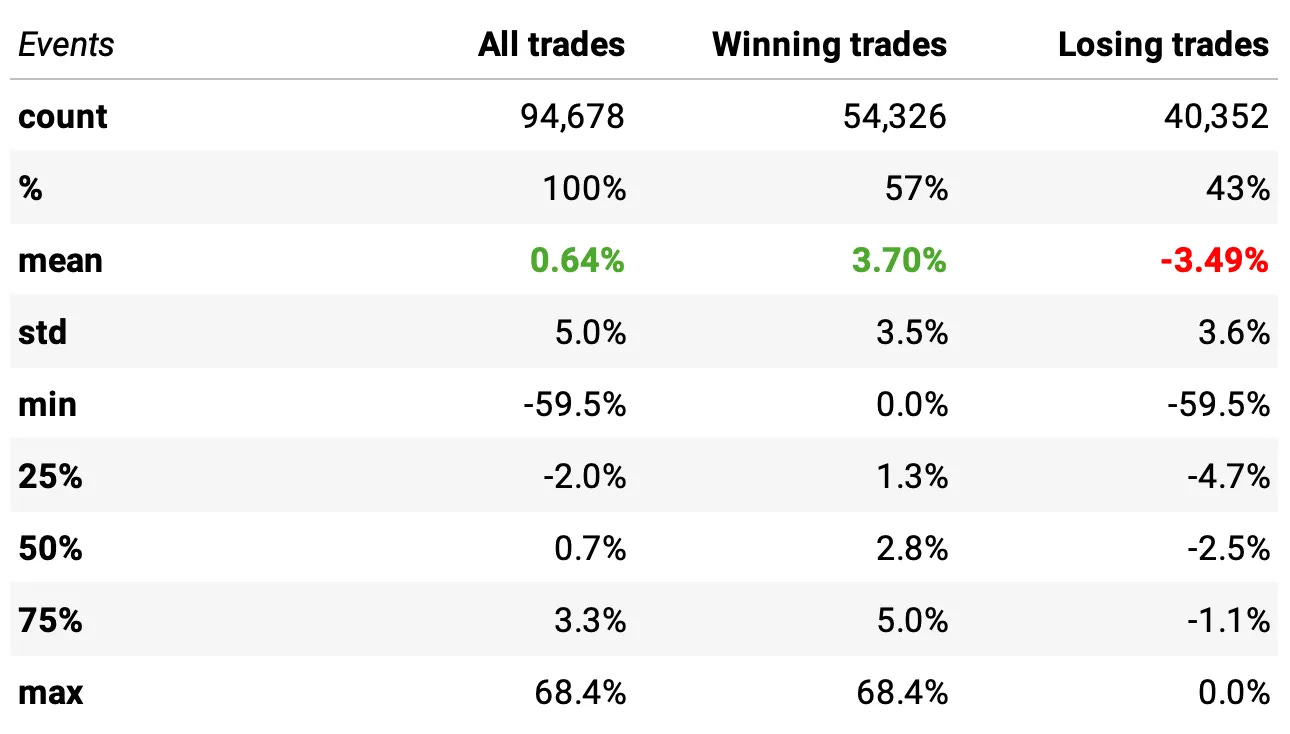
Win rate improved: 57% winners (vs. 57% before, but with a slightly better distribution of outcomes).
Expected return per trade increased: +0.64% per trade (vs. +0.60% in the baseline).
Winners were slightly stronger: average winner now +3.70% (vs. +3.60%), while losers remained roughly the same (–3.49%).
Statistically significant improvement: a statistical test shows the new return distribution differs from the baseline (t-stat = 3.37, p = 0.00062).
C) Improving the entry
The next improvement targets the entry signal itself. In addition to the existing conditions (a statistically significant price drop and the stock trading above its 200-day SMA), we now add one more filter: IBS (Internal Bar Strength). Specifically, we require IBS < 0.10, meaning the stock closed in the bottom 10% of its intraday range.
To keep the strategy supplied with enough trading opportunities, we also relax the QPI threshold from 0.15 to 0.30. After adding the stricter IBS filter, using the old QPI cutoff would make signals too scarce; widening it ensures we still capture a meaningful number of setups.
Why might this help? Because a large daily drop isn’t always enough to guarantee a good mean-reversion setup. Sometimes a stock bounces intraday, signaling buyers have already stepped in, which weakens the edge. By requiring IBS to be low, we target days where the stock was sold off all the way into the close, indicating persistent intraday pressure. These events tend to produce cleaner, more reliable snap-back behavior in the following days.
Let’s look at the data:
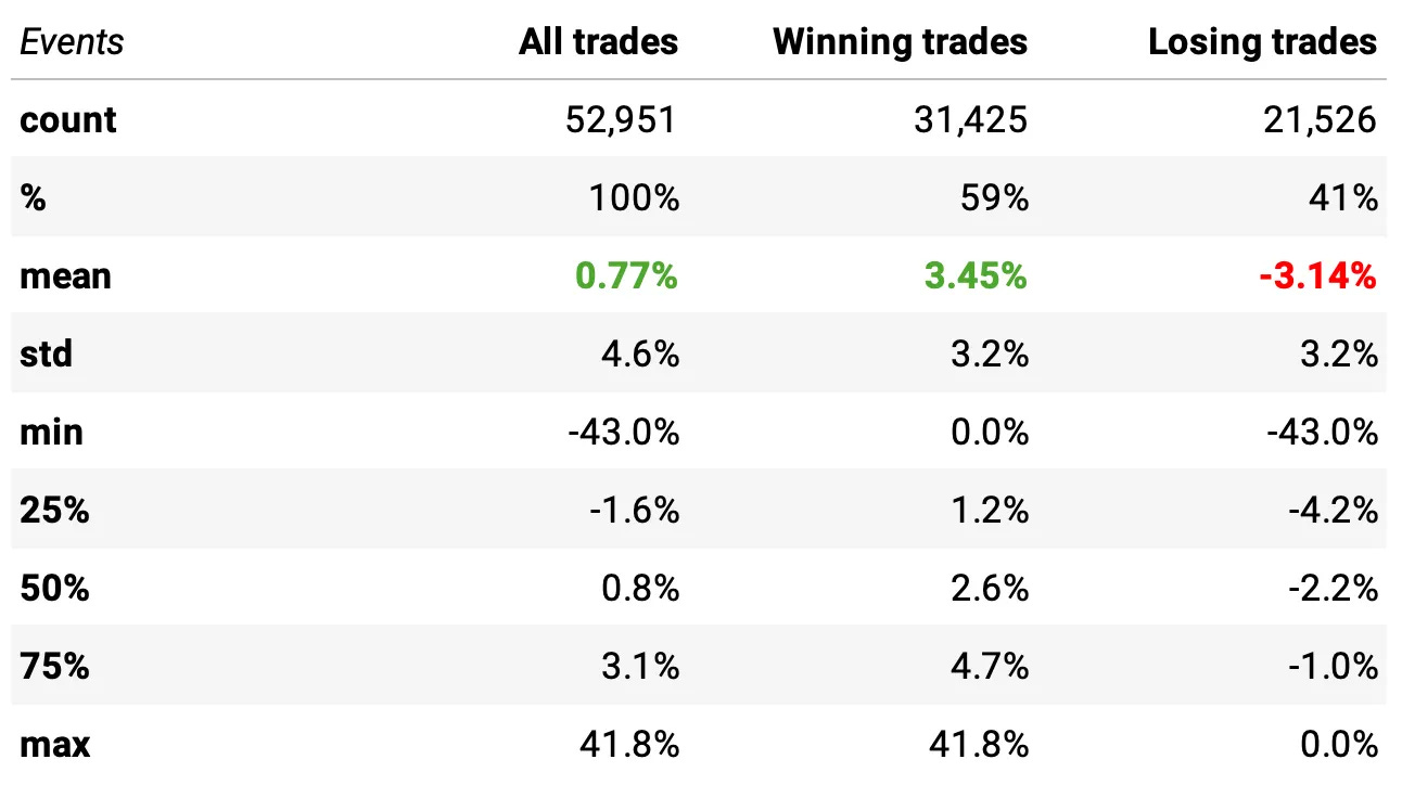
Win rate increased: 59% winners (up from 57% in the baseline).
Expected return per trade improved: +0.77% (vs. +0.60% in the baseline).
Winners stayed strong: average winner +3.45%, while losers averaged –3.14% (similar loss profile but with better selectivity).
Statistically significant improvement: a statistical test confirms the distribution is different from the baseline (t-stat = 8.32, p-value = 0.0).
D) Improving the exit
So far, we’ve been analyzing this signal using a time-based exit, holding each trade for exactly 5 days. But the actual strategy exits a trade as soon as today’s close is higher than yesterday’s high.
This makes intuitive sense: if you’re trading short-term mean reversion, the moment the stock snaps back above the prior day’s high, the “bounce” you were waiting for has already happened—there’s no reason to keep holding and expose yourself to further noise or new downside risk.
These are the stats with all improvements applied so far, using this exit logic:
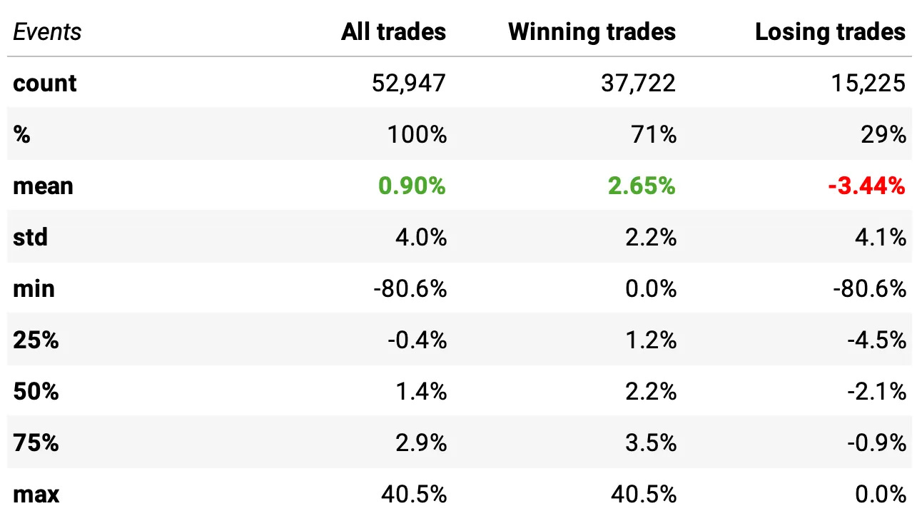
Win rate jumped significantly: 71% winners (up from 57% in the baseline).
Expected return per trade increased further: +0.90% (vs. +0.60% in the baseline).
Loss profile remained controlled: losers averaged –3.44%, while winners averaged +2.65% — a much healthier distribution.
Statistically significant improvement: a statistical test confirms this distribution is different from the baseline (t-stat = 14.38, p-value = 0.0).
But we can actually do better with exits. Instead of waiting for the price to break above yesterday’s high, we can test a more dynamic idea: closing the trade whenever IBS > 0.9 or RSI2 > 90.
Why might this work? Because both conditions signal exhaustion to the upside — when a stock surges into the top of its intraday range (IBS > 0.9) or becomes extremely short-term overbought (RSI2 > 90), the mean-reversion burst we were targeting has likely already played out. At that point, staying in the trade just adds noise and downside risk.
Let’s look at the data:
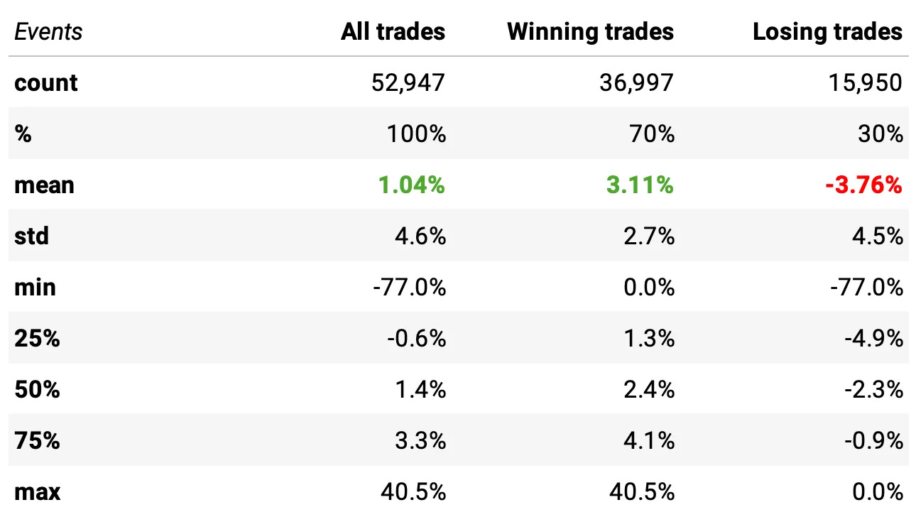
Expected return per trade improved further: +1.04% (up from +0.90% with the previous exit rule).
Win rate remained strong: 70% winners, with winners averaging +3.11% and losers averaging –3.76%.
Distribution remains healthy: median trade at +1.4%, with similar tail behavior but slightly better upside capture.
Statistically significant improvement: the distribution differs from the previous exit logic (t-stat = 5.37, p-value = 0.0).
Robustness
Before we move into walk-forward optimization, we first need to check whether the strategy is robust to reasonable parameter variation. To do that, we’ll test all 625 combinations from the following grid:
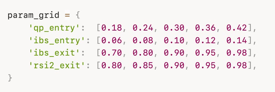
These ranges cover a wide and sensible portion of the parameter space—roughly 30–50% variation around each baseline value. Then,
If the strategy is truly robust, we should see stable performance across the grid—Sharpe ratios, annual returns, and drawdowns remaining positive and reasonably consistent across all 625 parameter sets.
If the strategy only performs well for a tiny handful of cherry-picked combinations, that’s a clear sign of fragility.
Before showing the results, it’s important to clarify the backtesting assumptions used throughout this robustness test (and in the walk-forward analysis that follows):
Increased diversification: we expand the maximum number of simultaneous positions from 4 to 10, as we previously discussed the importance of diversification.
Trading costs: each trade includes a 2 bps round-trip cost.
Equal-weighting: all trades are equal-weighted for simplicity and consistency across the 625 simulations.
Let’s see the data:
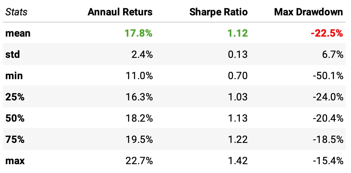
Robustness Results (2003–2025)
Annual returns are tightly clustered: median ≈ 18.2%, with most parameter sets between 16.3% and 19.5%.
Sharpe ratios remain consistently high: median ≈ 1.13, with 50% of all runs falling between 1.03 and 1.22.
Drawdowns are stable and controlled: median max drawdown ≈ –20%, with most runs between –24% and –18%.
No catastrophic parameter sets: even the worst combinations produce positive annual returns, Sharpe ≈ 0.70, and manageable drawdowns.
Is this a strong sign of robustness?
Yes. A strategy is robust when performance remains stable across a wide and reasonable part of the parameter space. Here, we tested 625 combinations, spanning roughly ±30–50% variation around each parameter. The results show:
No dependence on a narrow, cherry-picked parameter set
No sharp peaks or isolated “lucky” regions
A broad plateau of strong performance
Consistently attractive risk-adjusted returns (Sharpe ~1+) across the grid
Drawdowns that remain in a tight and acceptable range
This pattern — a large plateau of good solutions rather than a single spike — is exactly what we want to see in a strategy that is truly signal-driven rather than curve-fit.
Walk-forward optimization
Now that we’ve confirmed the strategy is robust across a wide range of parameter values, we face the next challenge: choosing which parameter combination to actually trade. If we simply pick the one that performed best on the full 2003–2025 dataset, we’d almost certainly be overfitting—rewarding parameters that benefited from historical noise rather than true predictive power.
This is where walk-forward optimization (WFO) comes in. Instead of optimizing on the entire dataset at once, WFO repeatedly trains the strategy on a rolling window of past data and immediately tests it on the next, unseen period. If a parameter set survives this sequence of “train → test → roll forward” cycles, it’s far more likely to capture a genuine, persistent edge that generalizes to real trading.
Walk-Forward Procedure
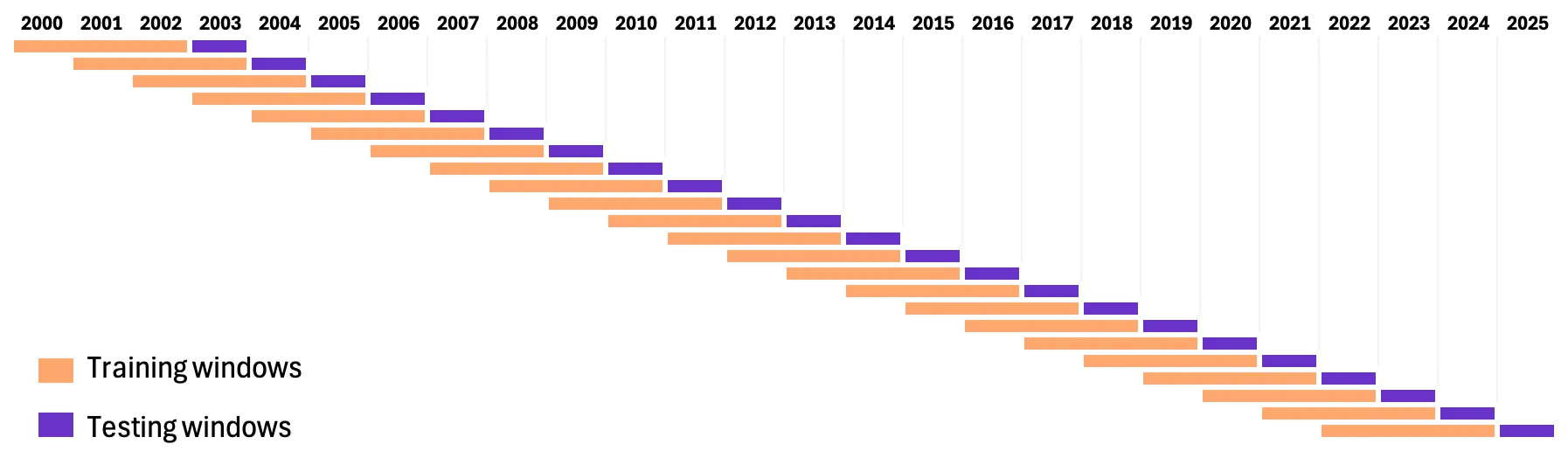
In our walk-forward framework, we use the following process:
3-year training windows:
For each step, we evaluate all 625 parameter combinations using only the previous 3 years of data.
Rank by Sharpe ratio:
Within each training window, we rank all parameter sets by their Sharpe ratio to identify the most stable performers.
Select the top 5 sets:
We take the five best-performing parameter sets and equal-weight them, effectively trading five independent portfolios as an ensemble.
Trade for the next year:
These five selected parameter sets are used to trade the following year, which serves as the out-of-sample test.
Roll forward one year:
After that year completes, we shift the entire window forward by one year and repeat the process:
train → rank → select → trade → roll.
Continue until 2025:
This rolling sequence continues until we reach the end of the sample, producing a full walk-forward performance series.
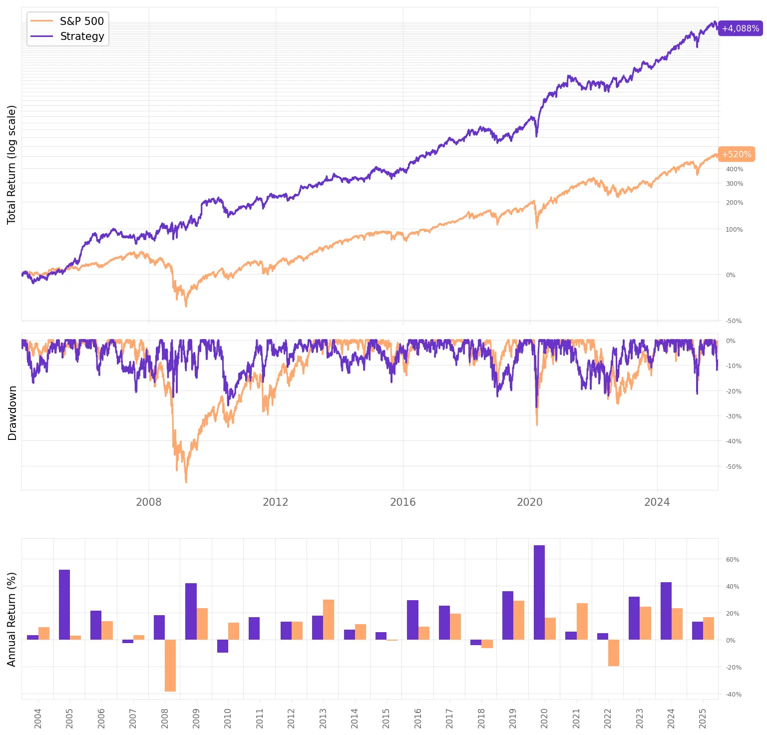
Results
With the walk-forward framework in place, we can now look at how the strategy performs out-of-sample:
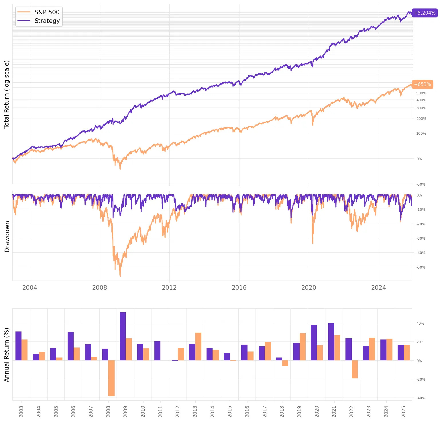
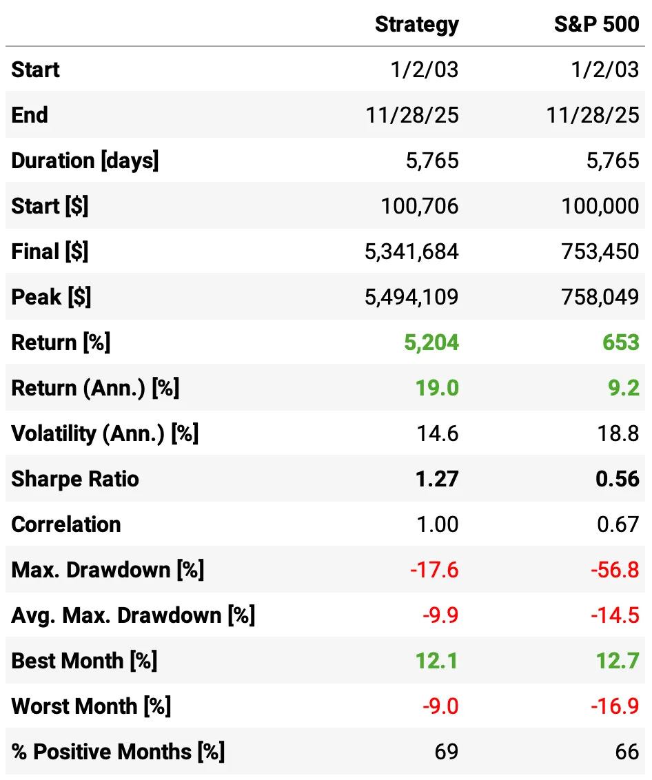
Final Strategy (after all improvements) vs. S&P 500:
Annual returns more than double the benchmark: 19.0% vs. 9.2% per year.
Sharpe ratio more than 2× higher: 1.27 vs. 0.56, despite slightly lower volatility (14.6% vs. 18.8%).
Significantly smaller drawdowns: 17.6% max drawdown vs. 56.8% for the S&P 500.
Smoother month-to-month performance: 69% positive months vs. 66% for the index.
Final Strategy vs. Original Flawed Strategy:
Sharpe ratio improved dramatically: from 0.90 → 1.27 (a 41% increase in risk-adjusted performance).
Volatility materially reduced: 14.6% vs. 21.6% — the improved version is much smoother.
Max drawdown cut from 26.8% to 17.6%
Better consistency: 69% positive months (final) vs. 62% (original).
About the same annual returns with less risk: 19.0% vs. 18.7%, but achieved with far lower volatility and far better drawdown behavior.
Now, let’s look at monthly and annual returns:
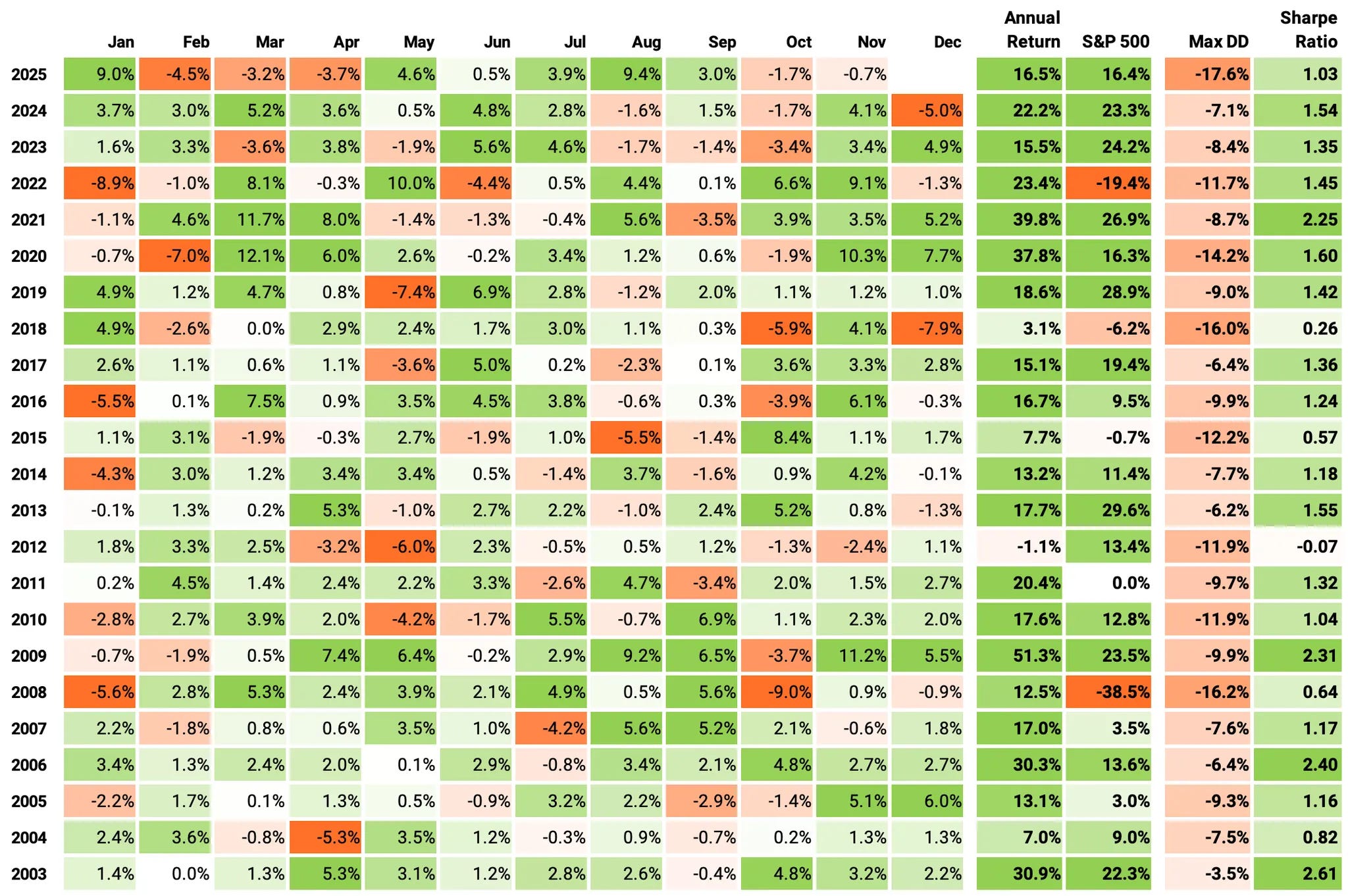
If we had traded this strategy since 2003:
We would have had only 1 down year in 22 years (2012);
We would have seen 69% of the months positive, with the best at +12.1% (Mar’20);
We would have seen 31% of the months negative, with the worst at -9.0% (Oct’08);
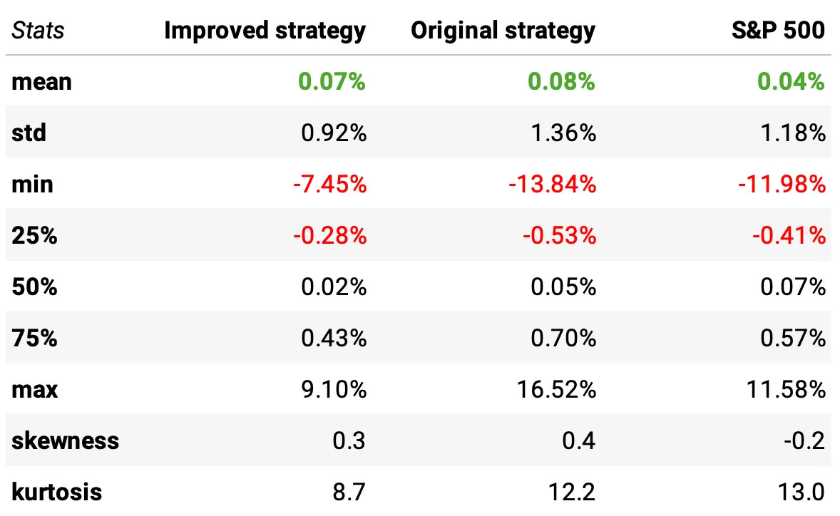
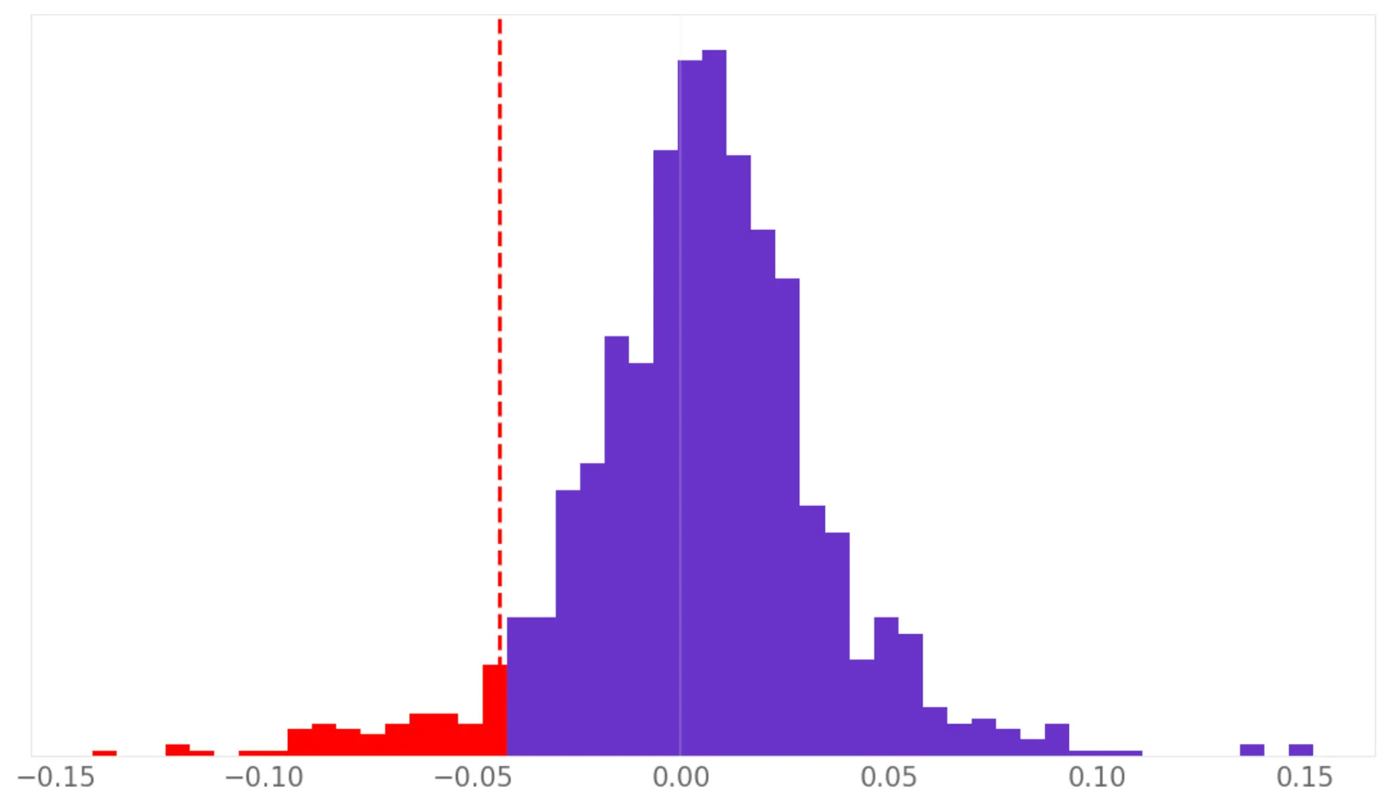
The table above compares the daily return distribution, and clearly shows what actually improved:
Volatility dropped by ~32% in the improved strategy (0.92% vs. 1.36%), producing a dramatically smoother day-to-day P&L profile than the original system (and even smoother than the S&P 500 (1.18%)).
Tail risk improved substantially: the worst daily loss shrank from -13.84% → -7.45%, a ~46% reduction. This is one of the clearest signs that the new entry/exit logic and walk-forward ensemble are filtering out dangerous setups.
Typical losing days are much smaller: the 25th percentile improved from -0.53% → -0.28%, cutting the size of routine down days nearly in half.
Extreme outcomes (both good and bad) were reduced: max daily gain fell (16.5% → 9.1%), but so did extreme losses. The improved strategy trades “hero days” for far better stability — exactly what long-term compounding prefers.
Kurtosis dropped sharply (12.2 → 8.7): the distribution became significantly less fat-tailed, meaning fewer outliers and far more predictable behavior.
Slightly lower skewness (0.4 → 0.3) supports the same point: fewer wild upside days and far fewer wild downside days.
Despite all the risk reduction, mean daily return remained essentially the same (≈0.07% vs. 0.08%). The improved strategy delivers similar drift with meaningfully lower risk — the formula for a higher Sharpe.
Final thoughts
Murphy’s line — “Anything that can go wrong, will go wrong” — felt brutally accurate for this particular system in November. A handful of AI-related names went against it at the worst possible time, and a strategy that looked fine on paper suddenly felt fragile.
But that month also did us a favor: it forced us to look again into this system and ask a better question:
If this can fail, where will it fail, and how do we design it so it doesn’t?
The answer wasn’t a single clever trick. It was a list of small, unglamorous improvements: tighter entries (IBS + relaxed QPI), more intelligent exits, trading at the close, parameter robustness checks, and a walk-forward process that refuses to lock in one lucky configuration. None of these changes is spectacular on its own. Together, they turned a decent but jumpy strategy into one that doubles the S&P’s return, cuts drawdowns by two-thirds, and delivers a much cleaner return distribution.
The main lesson for me is that robustness is something we build deliberately. What worked better here was treating the idea as a prototype and then pushing on it from all sides: testing hundreds of parameter sets, forcing it through walk-forward OOS, and quietly hardening all the places where Murphy could attack — entries, exits, sizing, and risk.
There’s still plenty to do. We haven’t yet touched the other two levers we identified:
Breadth/diversification — scaling to more slots and possibly more universes;
Risk overlay — hedging factor exposures (β, size, momentum, sector) so we’re less exposed to the kind of “AI repricing month” that triggered this whole review. I also want to explore ways of explicitly separating fundamental repricings from noise-driven dislocations, so we can avoid stepping in front of real information shocks.
If there’s a broader takeaway, it’s this: Murphy’s Law doesn’t have to be a curse. Treated correctly, it’s a design principle. Assume things will go wrong, and then build systems that still behave well when they do.
As always, I’d love to hear your thoughts. Feel free to reach out via Twitter or email if you have questions, ideas, or feedback.
Cheers!
Study Group
Our last study group was a success. Thank you to all community members who joined live! For those who couldn’t, I will post the code and the recording on learn.quantitativo.com, as usual, in the next few days. The TAA strategy we reviewed is up almost 40% this year.
Lately, our community has shown interest in a wide range of topics on the forum. As usual, I’ll post a survey on connect.quantitativo.com so everyone can vote on the topic for the next study group.
I know I said I would reopen enrollments in December… but I am completely swamped with work, so I’ll reopen enrollments in January 2026. The waitlist already has a few hundred people. Join it below to be the first to know when new seats open:
Impressive results.
This'd only work in the nutty world of the S&P where there are _very_ few meaningful downtrends.
1.what is QPI?
2.can you give a rough idea of the value of the drop threshold?
(at 3-5k-trades/yr it is likely <5%, either way perhaps a window of acceptable drops may weed out some large drops that will not recover.)
3. Should also try distribution of returns to be relative to the centroid (S&P index)
4.Since you hinted at it, how would you modify this for shorter time frames?
In my experience most academic papers don’t hold up in practice. However it gives insight into what shops are very likely investigating. Thanks for sharing!