Short-Term Basis Reversal
An anomaly that delivers a 1.45 Sharpe ratio and 19.2% annual returns


The idea
“A single hair from the head of a woman is worth more than all the books of Galen and Avicenna.” Paracelsus.
Paracelsus (1493–1541) was one of the most radical and influential physicians and philosophers of the Renaissance. A restless traveler, alchemist, and fierce critic of medical orthodoxy, he believed that true knowledge came not from ancient books but from direct observation of nature and practical experience.
Paracelsus helped shift medicine from being a theoretical, bookish discipline toward an experimental, empirical one.
I want to start by mentioning Paracelsus for two reasons. First, on a very personal note, I’m thrilled that my little brother just got into medical school! He’s going to be the first doctor in our family, and I couldn’t be prouder.
Second, I still remember my German chemistry professor in engineering school speaking of Paracelsus with great respect. As someone who valued experiment over theory, and real-world observation over books. In my view, that’s the heart of science: we trust what we test.
This week, we will implement the paper Short-Term Basis Reversal, by Alberto G. Rossi, Yingguang Zhang, and Yandi Zhu. In the paper, the authors devised a strategy that delivered 18% annual returns over several decades, with a Sharpe ratio of 1.42.
Can we replicate that? Let’s find out… because, as Paracelsus taught us, the true value of any idea lies not in how good it looks on paper, but in whether it holds up in practice.
Here’s the plan we will follow:
First, we will review the paper and summarize its main points.
Then, we will implement the strategy for a single market (time-series).
Next, we will implement the market-neutral strategy across all markets (cross-sectional).
Finally, we will discuss the next steps on how to execute.
Study Group
As mentioned in the article celebrating 1 year of Quantitativo, we are starting a Study Group via Zoom to review in-depth paper implementations. The first session will take place this Wednesday, June 11th, at 11 AM ET, and will be focused on this paper. I will share the connection details at connect.quantitativo.com.
Paper Summary
The paper discovers a new and significant anomaly in commodity futures markets: the short-term basis reversal: the return spread between adjacent futures contracts (e.g., front month vs. second month) shows strong negative autocorrelation week to week.
When the first-minus-second nearby contract return is high one week, it tends to reverse the next.
Core idea
In markets with a term structure (like futures curves), the front-month (F1) and second-month (F2) futures contracts often move together (but not perfectly).
Each week, the spread return between F1 and F2 (i.e., Return(F1) - Return(F2)) shows a strong tendency to reverse the following week.
If the spread was positive this week → likely negative next week (and vice versa).
This is called Short-Term Basis Reversal.
Why Does This Happen?
Front-month contracts (F1) are more liquid and adjust faster to new information.
Second-month contracts (F2) adjust more slowly (due to lower liquidity, less trading, preferred habitat of some market participants).
This creates temporary mispricings between F1 and F2.
Arbitrage capital is slow-moving → mispricings persist 1-2 weeks → predictable reversals.
How to Exploit It
Each week, look at the previous week’s spread return (Return(F1) - Return(F2)):
If spread was strong positive → expect reversal → next week spread likely negative
If spread was strong negative → expect reversal → next week spread likely positive
There are two ways to trade this effect:
1. Time-Series Strategy (Single Market)
For each commodity individually:
If its spread return was positive last week → trade short spread this week
If its spread return was negative last week → trade long spread this week
Works in 18 of 22 commodities → high Sharpe, robust
2. Cross-Sectional Strategy (Multiple Markets)
Each week, rank all 22 commodities based on their prior-week spread return
Go:
Long spreads of the 4 commodities with most negative prior spread return (expect reversal up)
Short spreads of the 4 commodities with most positive prior spread return (expect reversal down)
Portfolio holds 8 spreads (16 contracts total)
Delivers even higher Sharpe (up to 1.42) — scalable and more diversified
This is the gist of the paper. I strongly recommend reading it, especially for those participating in the study group. Now, let’s look at the implementation results for a single market.
Time-Series Strategy Results (Single Market)
We use Norgate Data, which is a different data source from the one the authors used in the paper.
Norgate provides daily data for 39 different commodity markets, across Agriculture (26), Energy (8), and Metals (5).
To test the simpler strategy (time-series in a single market), we will focus on Feeder Cattle futures (GF).
I will share the code and detailed implementation in the study group. But it is straightforward. The key is to create a table that, for each week, show the exact first-month and second-month contracts. Then, retrieving the prices, computing returns and the spread is pretty simple.
IMPORTANT: When the authors define first-nearby contract, it is the first eligible contract with at least 1 month to expiration, not simply the calendar first-month contract.
Here are the results:
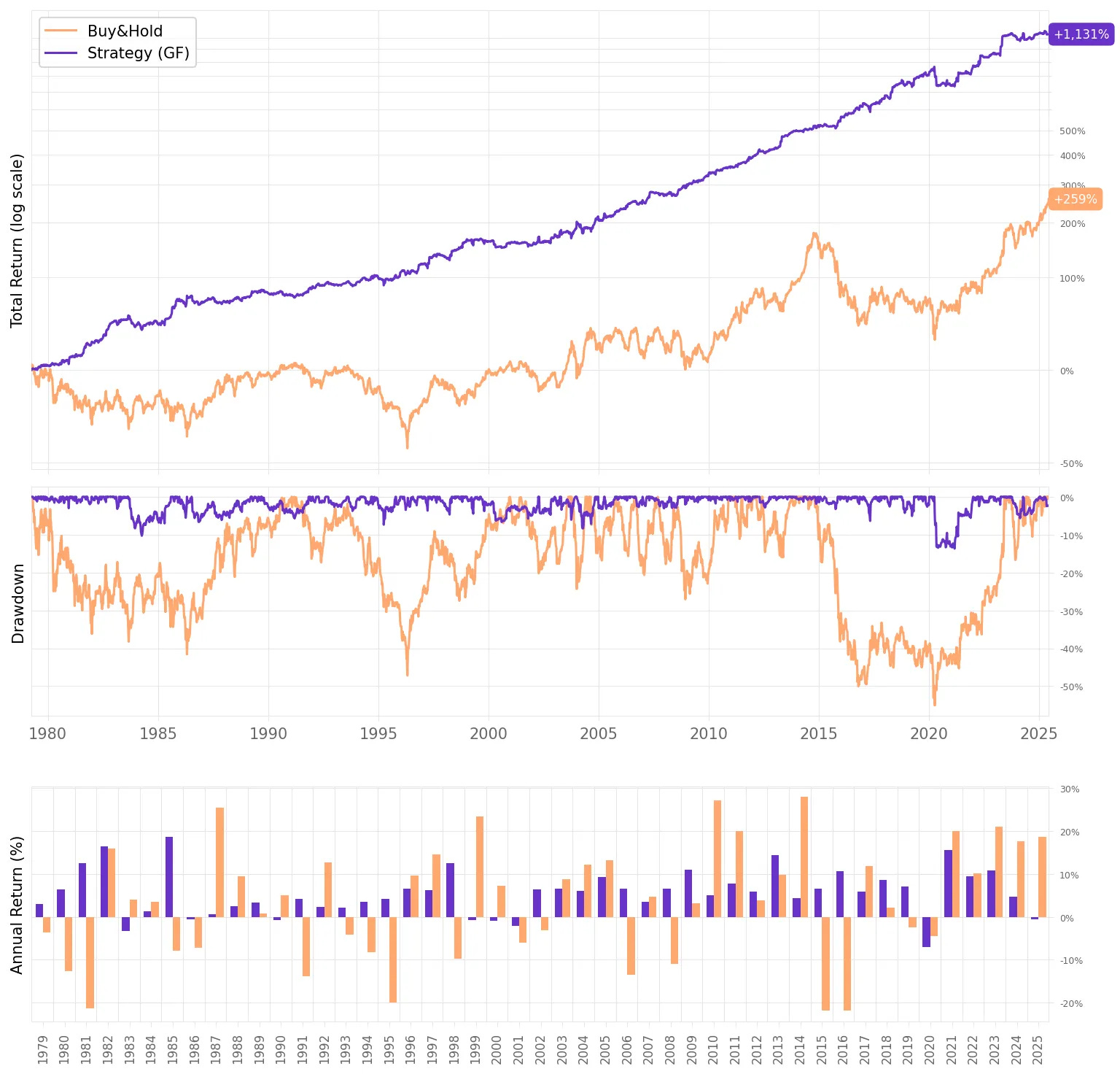
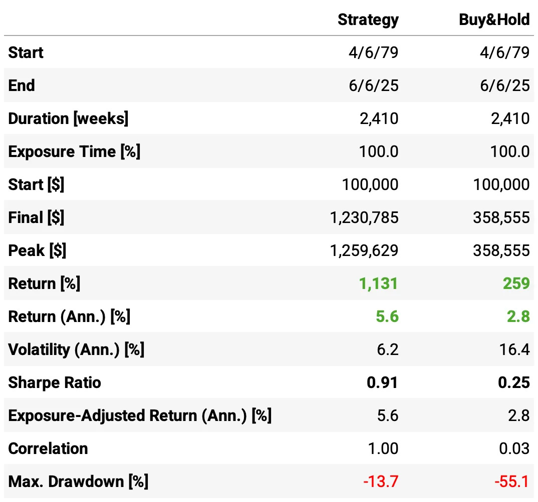
Quite a strong result. This would have outperformed Buy & Hold convincingly:
Annual return is +5.6% vs. 2.8% Buy & Hold;
Sharpe ratio is 0.91, more than 3x better than Buy & Hold’s 0.25;
Max drawdown is very controlled at -13.7% vs. a painful -55.1% for Buy & Hold;
Volatility is also much lower: 6.2% vs. 16.4%;
Finally, note the almost no correlation to Buy & Hold (0.03).
Now, let's look at the cross-sectional strategy.
Cross-Sectional Strategy Results (Multiple Markets)
Now that we've tested the strategy in a single market, we move to the full cross-sectional version. In this step, we apply the strategy across all 39 commodity markets available in Norgate Data, spanning Agriculture, Energy, and Metals. The table below lists the full set of markets considered in our implementation.

Visualizing the edge
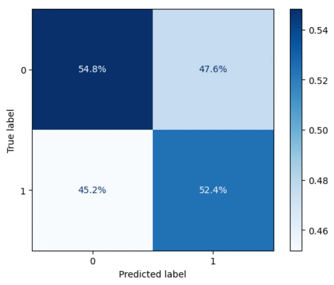
As a simple diagnostic, before looking into the strategy backtest, let's check whether the strategy correctly predicts the direction of the spread return from week to week. The confusion matrix below shows the results (1 for positive/long weeks, 0 for negative/short weeks). The overall accuracy is 53.6%, above the 50% baseline expected from random guessing.
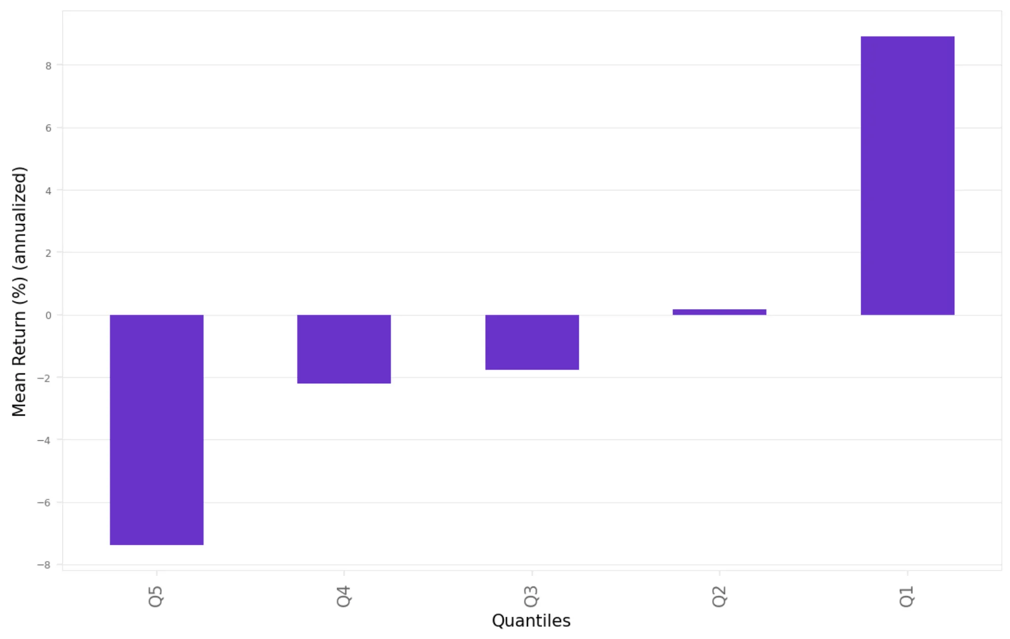
To visualize the edge more clearly, we classified the spread returns into quintiles based on the predicted signal and aggregated the realized returns for each group. The chart below shows the annualized mean return for each quintile. As we can see, the results display a clear monotonic pattern. The most extreme predicted spreads (Q1 and Q5) show the strongest directional returns, which highlights the predictive power of the signal.
Backtesting the strategy
Now, let’s backtest the long&short market neutral strategy. The core idea is straightforward:
Each week, we rank all 39 commodities based on their spread return from the previous week.
We then take positions as follows:
Go long the spreads of the 4 commodities with the largest negative spread returns (anticipating a rebound).
Go short the spreads of the 4 commodities with the largest positive spread returns (anticipating a reversal lower).
Here are the results:
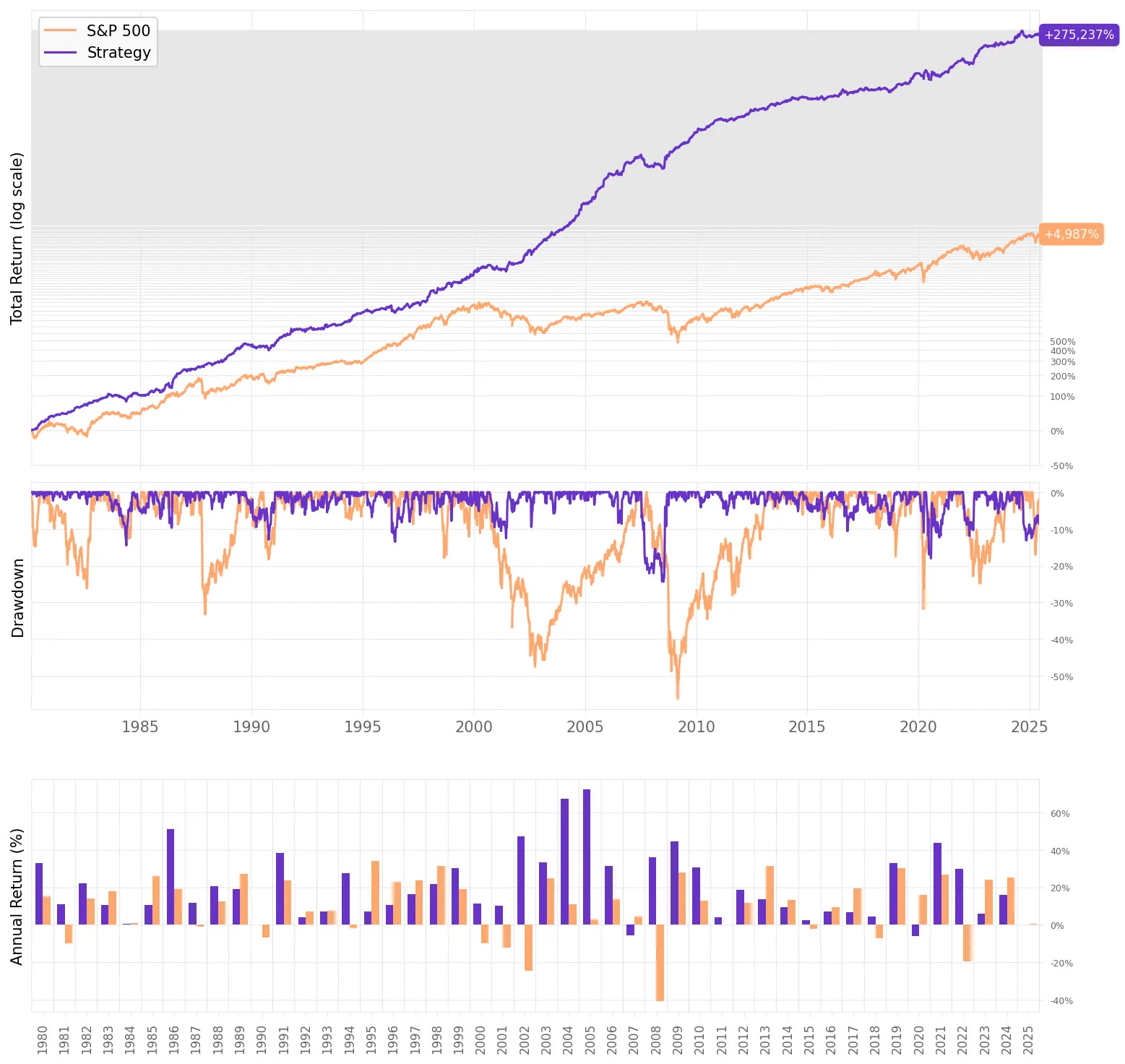
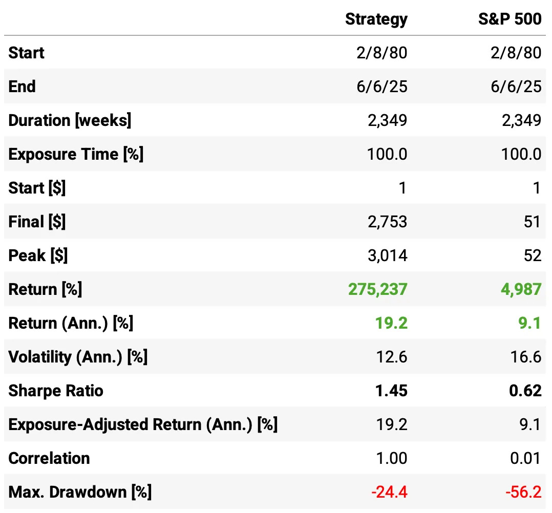
We can see a strong performance for the cross-sectional strategy:
Annual return is 19.2%, more than 2x the S&P 500’s 9.1%;
Sharpe ratio is good at 1.45, vs. 0.62 for the benchmark;
Max drawdown is well controlled at -24.4%, while the benchmark suffers a brutal -56.2%;
Volatility is also lower than S&P 500: 12.6% vs. 16.6%;
And (as expected for a market-neutral approach) the strategy has virtually zero correlation with the S&P 500 (0.01).
Now, let's see how the trading costs impact the strategy.
Impact of Trading Costs
We have assumed 10 bps of trading costs, deducted weekly. Let’s now examine how different levels of trading costs affect the results:
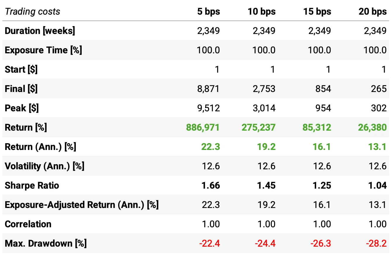
As expected, trading costs have a significant impact on the strategy's performance. However, the edge remains robust even with higher cost assumptions:
With 5 bps of costs, the strategy delivers an excellent 22.3% annual return and a 1.66 Sharpe;
At 10 bps (our base case), results are still very strong: 19.2% annual return and 1.45 Sharpe;
Even at 15 bps and 20 bps, the strategy remains profitable (Sharpe stays above 1), though returns naturally compress: 16.1% and 13.1% annual returns, respectively;
Importantly, max drawdown remains stable across cost levels (around -22% to -28%), indicating the strategy does not become more fragile as costs rise.
Impact of Number of Spreads
In our base case, we traded 8 spreads (4 long, 4 short). Let’s now examine how changing the number of spreads affects the results:
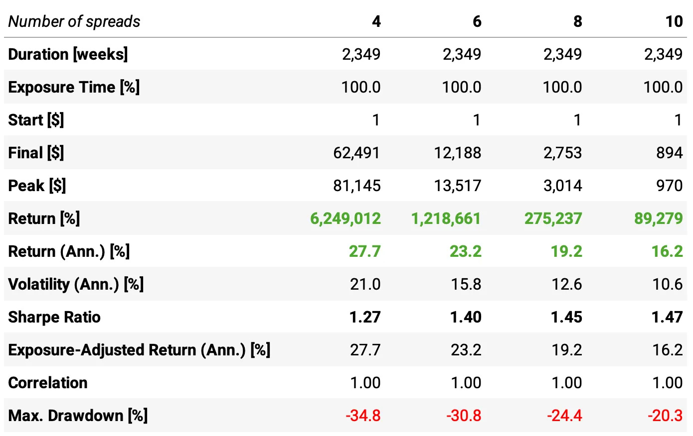
As we vary the number of spreads, we observe a clear trade-off between return and risk concentration:
Using only 4 spreads maximizes returns (27.7% annually) but comes with very high volatility (21%) and large drawdowns (34.8%);
Increasing to 6 spreads improves Sharpe (1.40) while reducing risk somewhat, though returns drop to 23.2% annually;
The base case (8 spreads) shows the best risk-adjusted profile: Sharpe 1.45, volatility 12.6%, max drawdown 24.4%, with a still strong 19.2% return;
Adding more spreads (10) further stabilizes the strategy (lowest volatility, lowest drawdown), but at the cost of reduced returns (16.2%), possibly due to diluting edge across weaker-ranked markets.
In short: the 8-spread configuration appears to offer the best balance between performance and robustness.
Final Thoughts
The implementation of this paper will be a great way to kick off our Quantitativo Study Group this Wednesday. It’s a clean example of how a simple empirical anomaly, when rigorously tested and thoughtfully implemented, can translate into a potentially robust trading strategy.
The Short-Term Basis Reversal strategy not only held up out-of-sample, but also performed better than in the original paper, especially when implemented as a cross-sectional market-neutral portfolio.
Starting from a simple empirical observation about spread reversals in commodity term structures, we built a scalable and robust trading strategy. Even after factoring in trading costs and varying the number of spreads, the edge remained strong: Sharpe ratios above 1, strong annual returns, and controlled drawdowns.
A few takeaways stood out:
The edge is surprisingly consistent across markets and over time;
The cross-sectional version offers the best risk-adjusted profile, while also being more scalable;
The signal shows a clear monotonic relationship with realized returns, suggesting it captures a real and persistent structural inefficiency.
Of course, this was still a baseline test. There is plenty of room for further exploration:
Should we dynamically adjust the number of spreads traded based on market conditions?
Could we optimize the selection and sizing of spreads (e.g., using advanced ranking, volatility scaling, or ensemble signals)?
How well does this edge hold up with intraday data or shorter rebalancing cycles?
This is the spirit of Paracelsus: trust what you test, and always experiment further. The results so far are very encouraging.
As always, I’d love to hear your thoughts. Feel free to reach out via Twitter or email if you have questions, ideas, or feedback.
Cheers!
The first cohort of the course was a great success. Thank you to everyone who joined!
Enrollment is now closed. The next cohort opens in August, with 50 more seats.
Course participants also get exclusive access to our Community and Study Group.
Join the waitlist below to be notified when enrollment reopens:
(I know, I need to update this landing page… as soon as I find time I will add more details about the course, the community, reviews from the 50 first users, etc :))
I’m not able to produce these returns after associating cost (10bps) per basis. It completely destroy lies the returns.
A 1.45 Sharpe and 19% returns on a basis reversal will always make for great reading, but let’s keep it honest: by the time an edge hits Quantitativo or Substack, it’s already being gnawed on by every quant desk from Chicago to Singapore.
Pietro nailed it in the comments: if your backtest relies on settlement prices, not what you can actually fill in the real market, you’re living in a spreadsheet fantasy.
The theory is sharp, but live trading means slippage, roll costs, and a crowd of faster, bigger players all chasing the same ghost. Test small, measure what you really get (not what the backtest promises) and remember, the best edges never see the light of day.